![]() Clara V. Teixeira-Leite1
Clara V. Teixeira-Leite1 ![]() and
and ![]() Marcelo Vianna1
Marcelo Vianna1
PDF: EN XML: EN | Supplementary: S1 S2 | Cite this article
Abstract
Biodiversity baselines are essential subsidies to evaluate how environmental changes and human impacts affect the special and temporal patterns of communities. This information is paramount to promote proper conservation and management for historically impacted environments such as Guanabara Bay, in southeastern Brazil. Here, we propose an ichthyofaunal baseline for this bay using gathered past data from 1889 to 2020, including literature records, scientific collections, biological sampling, and fisheries landing monitoring. A total of 220 species (203 teleosts and 17 elasmobranchs), distributed in 149 genera (136 teleosts and 13 elasmobranchs) and 72 families (61 teleosts and 11 elasmobranchs) were recorded, including the first record of a tiger-shark, Galeocerdo cuvier, in Guanabara Bay. Although the employed sampling effort was sufficient to represent the ichthyofauna in the middle and upper estuary, the Chao2 estimator indicates an even greater richness regarding the bay as a whole. Evidence of reduced abundance and probable local extinction over the decades was found, supporting the importance of implementing management and conservation strategies in the area. The ichthyofaunal distribution analyses revealed that areas close to conservation units are richer compared to their surroundings, indicating that this is an effective strategy to mitigate human impacts in the bay.
Keywords: Brazil, Inventory, Scientometric review, Species density, Tropical estuary.
Esforços de caracterização da biodiversidade são subsídios essenciais para avaliar como mudanças ambientais e impactos antrópicos afetam os padrões espaciais e temporais das comunidades. Essas informações são essenciais para promover conservação e manejo adequados em ambientes historicamente impactados como a Baía de Guanabara, no sudeste do Brasil. Aqui, nós propomos uma linha de referência da ictiofauna dessa baía utilizando dados pretéritos de 1889 a 2020, incluindo registros de literatura, coleções científicas, coletas biológicas e monitoramento de desembarque pesqueiro. Um total de 220 espécies (203 teleósteos e 17 elasmobrânquios), distribuídas em 149 gêneros (136 teleósteos e 13 elasmobrânquios) e 72 famílias (61 teleósteos e 11 elasmobrânquios) foram registradas, incluindo o primeiro registro de tubarão-tigre, Galeocerdo cuvier, na Baía de Guanabara. Apesar do esforço amostral empregado ter sido suficiente para representar a ictiofauna do médio e alto estuário, o estimador Chao2 indicou uma riqueza ainda maior para a baía como um todo. Evidências de redução de abundância e de provável extinção local de táxons ao longo das décadas foram encontradas, corroborando a importância da implantação de medidas de manejo e conservação para a área. A análise da distribuição da ictiofauna revelou que áreas próximas a unidades de conservação são mais ricas em comparação ao seu entorno, indicando que essa é uma estratégia efetiva para mitigar os impactos antrópicos na baía.
Palavras-chave: Brasil, Densidade de espécies, Estuário tropical, Inventário, Revisão cientométrica.
Introduction
Estuaries are highly dynamic coastal environments that exhibit a wide range of salinity, nutrient, and temperature variations, providing habitats, resources, and shelter to a variety of species at different life cycle stages (Silva-Junior et al., 2016; Wolanski, Elliott, 2016). Estuaries function as important nursery and feeding areas (Corrêa, Vianna, 2015; Santos et al., 2015; Andrade et al., 2016; Mérigot et al., 2017; Gonçalves-Silva, Vianna, 2018b), which are essential for the maintenance of several marine fish stocks (Santos et al., 2020). Even though these environments are known to contain few strictly resident species (Andrade-Tubino et al., 2008; Vianna et al., 2012; Silva-Junior et al., 2016; Gonçalves-Silva, Vianna, 2018a), their ichthyofaunal diversity displays a rich taxonomic composition, including many species of economic interest and others at serious risk of extinction.
The Guanabara Bay is the second largest Brazilian estuary, located in the metropolitan region of the state of Rio de Janeiro, presenting significant historical, environmental, touristic, and scenic importance. The bay also comprises an essential part of Rio de Janeiro’s economy, since it harbors a major port area and supports the most productive estuarine fisheries in the region (Prestrelo, Vianna, 2016). Guanabara Bay has historically suffered from a series of human impacts associated to huge solid waste, untreated domestic sewage, and persistent pollutant inputs, such as metals and hydrocarbons (Pereira et al., 2007; Rosenfelder et al., 2012; Silva-Junior et al., 2012, 2016; Hauser-Davis et al., 2019a; Paiva et al., 2021). Despite several impacts, this estuary is still ecologically relevant and is considered an area with the potential to become a priority for Brazilian conservation according to guidelines of the Brazilian National Biodiversity Commission (Teixeira-Leite et al., 2018).
Guanabara bay’s ichthyofauna is historically a common target of scientific studies (e.g., Gomes et al., 1974; Toledo et al., 1983; Brum et al., 1995; Brum, 2000; Baêta et al., 2006; Vasconcellos et al., 2010; Mulato et al., 2015) as many research centers are located around the bay (e.g., Universidade Federal do Rio de Janeiro, Universidade Federal do Estado do Rio de Janeiro, Universidade Federal Fluminense, Universidade do Estado do Rio de Janeiro). However, knowledge on several aspects of the bay’s biodiversity was dispersed over the years in different literature, hindering a more comprehensive understanding of the bay’s fish diversity. Reliable and informative inventories are important to promote the conservation and adequate management of natural areas (Reis-Filho et al.,2010; Silveira et al., 2010; Sreekanth et al., 2020), in addition to providing a baseline to assess how environmental changes and human impacts affect temporal community variations (Sheaves, 2006). Vianna et al. (2012) made a first attempt to gather past knowledge of the bay’s ichthyofauna by developing a list of local species, but most of the information they recovered was not based on published articles that went through proper critical peer-review. In addition, since 2012 new research initiatives that monitor experimental collections and fishing landings carried out by research groups (e.g., Laboratório de Biologia e Tecnologia Pesqueira – BioTecPesca/UFRJ, Universidade Federal do Rio de Janeiro) have promoted a considerable increase in knowledge concerning the ichthyofauna of the bay.
The aim of this study is therefore to develop a baseline of Guanabara Bay’s ichthyofauna, to achieve a better understanding of the composition, distribution, and richness of fish species in the bay. The use of reliable past data (e.g., articles published in indexed journals, voucher specimens deposited in ichthyological collections, biological samplings and fishing landings monitored by BioTecPesca/UFRJ) make this inventory a basis for comparison for future studies. It also potentially reveals changes in species composition that have already taken place throughout history.
Material and methods
Study area. TheGuanabara Bay (22°59’02.20’’S – 22°40’23.66’’S; 43°01’26.53’’W – 43°17’26.08”W) is a semi-enclosed tropical estuary located on the southeastern coast of Brazil, in the state of Rio de Janeiro, covering 384 km2, with an average volume of 1.87 x 10⁹ m3 of water, and a 4,080 km2 drainage basin with maximum depth of 50 m in the central channel (Meniconi et al., 2012; Silva-Junior et al., 2016). It is characterized by seasonal salinity variations influenced by a connection with oceanic waters, the local rainfall regime, and tides. During the low rainfall period (June to August), the water column is more homogeneous, with little temperature and salinity variations, becoming vertically stratified during the rainy season (December to March), with the appearance of upwelling areas due to the penetration of the South Atlantic Central Water (SACW) that enters the estuary through its saline wedge (Valentin et al., 1999; Silva-Junior et al., 2016).
The bay is categorized into three compartments (sensu Silva-Junior et al., 2016; Souza, Vianna, 2022): (i) the lower estuary, corresponding to the central channel and its banks, comprising the area suffering the greatest influence of the oceanic waters that enter the bay; (ii) the middle estuary, consisting of an intermediate transition area between the more saline waters of the lower estuary and the more brackish waters of the upper estuary, and (iii) the upper estuary, the innermost bay region under greater influence of continental waters from the local hydrographic basin.
The Guanabara Bay entrance was defined as the shortest distance between the east and west coasts (limit line, from the point of Forte São José, 22°56’24.41”S 43° 09’06.66”W to the point of Fortaleza de Santa Cruz da Barra, 22°56’16.97”S 43°08’06.30”W). Therefore, all records external to this line were considered as outside the estuarine region and were not included in our inventory. The bay was also divided into quadrants using the Quantum GIS (QGIS) software version 3.16.5 according to the same grid applied by the fishing landing monitoring efforts in Guanabara Bay (Prestelo, Vianna, 2016) (Fig. 1).

FIGURE 1| Guanabara Bay map, Rio de Janeiro, divided into five km x five km quadrants. Different shades of blue indicate which estuary compartment (upper, middle or lower) the quadrant belongs to.
Data compilation. Different strategies were employed to gather ichthyofaunal records in the Guanabara Bay. First, we made a compilation of scientific literature concerning the bay’s ichthyofauna. A scientometric analysis was carried out at the Web of Science, SciELO and Scopus portals, covering articles from all available years, i.e., from 1921 to March 23, 2021. The search method applied two keyword fields linked by the connectors “AND” and “OR”, the first referring to the study location (Guanabara Bay) and the second to the study group (ichthyofauna) (Tab. 1). We added to the scientometric analysis results other published articles that were previously known by the authors. Then, data from two sets of fish samplings carried out by BioTecPesca/UFRJ were added to the database. These bottom trawl samplings were carried out from 2005 to 2007 at quadrants C3, C5, D5, D7, E3, E5 and E7; and from 2013 to 2015 at quadrants C5 and D5. In addition, the records of species identified in two artisanal fishing landing monitoring programs at Guanabara Bay based on different commercial fishing gear (also carried out by BioTecPesca/UFRJ) were considered, the first in 2009 and 2010, and the second in 2013 and 2014.
TABLE 1 | Keywords used in the scientometric search on fish at Guanabara Bay, Rio de Janeiro.
Keywords | |
1º search field | “Guanabara bay”
OR “Guanabara” OR “baía de Guanabara” OR “bahía de
Guanabara” |
“AND” 2º search
field | “fish*” OR “teleost*” OR “elasmobran*” OR “pisces” OR “shark*”
OR “ray*” OR “stingray*” OR “chondrichth*” OR
“skate*” OR “bone fish*” OR “agnatha*” OR “osteichthy*” OR “actinopter*”
OR “peixe*” OR “pesca*”
OR “elasmobrânqui*” OR “tubar*”
OR “raia*” OR “arraia*”
OR “condrict*” OR “agnat*”
OR “osteíct*” OR “pez” OR
“tiburón” OR “tiburones”
OR “raya*” |
Historical records were obtained from the online databases of the fish collections of Museu de Zoologia da Universidade de São Paulo, São Paulo (MZUSP) (records available online at https://mz.usp.br/pt/laboratorios/ictiologia/ accessed on July 30, 2020) and the Museu Nacional, Universidade Federal do Rio de Janeiro, Rio de Janeiro (MNRJ) (records available online at https://ipt.sibbr.gov.br/mnrj/resource?r= mnrj_ictiologia, accessed on July 30, 2020). In addition, we included to our data compilation the listings made by the BioTecPesca/UFRJ research group deposited at the Coleção de Peixes do Instituto de Biodiversidade e Sustentabilidade, Universidade Federal do Rio de Janeiro (NPM). The SpeciesLink Network (http://www.specieslink.net/) was used as another tool to compile records from several scientific collections. “Guanabara” was employed as keyword and the records were filtered by taxon to include only fishes, considering all reports until July 21, 2020. All lot numbers of species included in our database are available in Tab. S1.
Regardless of the strategy employed, records were considered only at the species level, with species without previous confirmed records in the state of Rio de Janeiro considered as doubtful records and not included in the baseline. Records at genus or family level were also not considered. Taxonomic classification (at species level and above) and species known distribution followed the Eschmeyer’s Catalog of Fishes (Fricke et al., 2023). As this study comprised only the Guanabara Bay, records obtained from local watershed rivers were not considered. Records from ichthyoplankton studies were also not included in our compilation. The historical baseline was built on data available until 2020, therefore we did not include records made after this year. However, we added the information of a few records made after this time-period in the Results section due to their ecological relevance. These include the first record of Galeocerdo cuvier (Perón & Lesueur, 1822) in Guanabara Bay and records of species that had not been recorded in the last decade (Bagre bagre (Linnaeus, 1766)) and Rhizoprionodon lalandii (Valenciennes, 1839)).
The selected records were used to build a baseline containing the currently valid name of the species, the year of the record, and the quadrant or quadrants where the species was recorded, if the information was available. When the exact year of collection was not indicated, the year of publication of the reference was considered as the date of the record. To generate a more complete inventory, the FishBase platform (https://www.fishbase.se) and specific literature on each species were used to obtain information on (i) feeding and functional guilds in the estuary (standardized according to Elliott et al., 2007) and (ii) habitat (standardized according to Silva-Junior et al., 2016). Finally, information on the extinction risk of each species was considered at both the global and Brazilian level, according to the IUCN Red List of Threatened Species (http://www.iucnredlist.org) and the Livro vermelho da fauna brasileira ameaçada de extinção (Subirá et al., 2018), respectively.
Data analysis. One of the main difficulties of studies that aim to assess the species richness of a given locality is to determine whether the employed sampling effort was sufficient to accurately estimate the richness (Schilling et al., 2012). As our study consisted on building a reference database using previously generated data, the number of sources consulted was considered as a unit of sampling effort. Thus, four absolute richness accumulation (S) curves by effort were constructed using the R software version 3.6.0, considering one for the bay as a whole and one for each of the three compartments of its estuary (low, medium and upper). In all cases, the random sample-based rarefaction method was used (Gotelli, Colwell, 2001) employing 100,000 permutations. In order to further understand the results of the curves, the non-parametric estimator for incidence data Chao2 was applied to each curve (Chao et al., 2009) which, in addition to allowing the verification of curve stabilization (reaching an asymptote), also provides a series of other information (Tab. 2). One of the advantages of using this estimator is the possibility to obtain “mg” values, since “g” values can be converted into percentages. In this context, if for a given “g” value extra collections are not necessary (null mg), then it is confirmed that the study in question was able to record the “g” of the percentage of total richness. A graph was also constructed for each rarefaction curve, where the x axis corresponds to “g” values and the y axis, to “mg” values.
TABLE 2 | Variables related to the non-parametric Chao2 estimator. The t, T, S obs, Q1 and Q2 values are used to calculate S est, q0, m and mg.
Variables | |
t | Number of
sources |
T | Total number of
incidences |
S obs | Number of
observed species |
S est | Number of
species estimated at the curve’s
asymptote |
Q1 | Number of
simpletons (species recorded by only
one source) |
Q2 | Number of
dobletons (species recorded by only
two sources) |
q0 | Probability of finding a new species if one
more source was consulted |
m | Number of
extra sources necessary to obtain S obs
= S est |
mg | Number of
extra sources necessary to obtain a proportion
“g” of the estimated richness (S est), with “g” ranging from 0 (representing 0% of S est) to 1 (representing 100% of S est) |
Concerning the spatial richness distribution, accumulation of absolute richness (S) values of each water quadrant was plotted on the bay map employing the QGIS software version 3.16.5. As each quadrant has its own water surface area (discounting portions of land, such as islands and coastlines), species density (S/water surface area) was also calculated in each one of them to obtain comparable results.
Finally, considering the bay’s history of environmental degradation and fishing exploitation, we expected the ichthyofaunal composition to change over the years. In this context, the temporal range of our baseline (1889 to 2020) was divided into decades to identify species that no longer occur in the bay, or that are at least rare now. We considered recent all records made from 2010 to 2020, because since 2010 there were no one-off impact events (e.g., oil spills) that may have affected the ichthyofaunal composition. Therefore, for this study purposes, the 10 years period between 2010 and 2020 (last decade) represent the recent state of the bay.
Results
Ichthyofauna richness and composition. The scientometric analysis resulted in a total of 176 published articles, 70 of which fitted the criteria described in Data compilation and were included in this study. Assembling all data compilation strategies, we considered a total of 84 different data sources. A total of 220 species (203 teleosts and 17 elasmobranchs) were recorded, distributed in 149 genera (136 teleosts and 13 elasmobranchs) and 72 families (61 teleosts and 11 elasmobranchs) (Tab. 3). Regarding the Teleostei, a very asymmetrical richness distribution was noted among families given that 14 families make up about 50% of the total recorded richness. Among these, the Sciaenidae included the highest number of species (23), followed by Carangidae (14) and Haemulidae (8). Concerning elasmobranchs, the numerical variation of species between families was lower, with the Dasyatidae and Carcharhinidae including three species each, followed by Sphyrnidae and Rhinobatidae with two species. Other families of the Elasmobranchii are represented by just one species each.
TABLE 3 | Species reported at Guanabara Bay and the sources, record dates and quadrants (column Q) in which these records occurred. Taxonomic classification (at species level and above) followed the Eschmeyer’s Catalog of Fishes (Fricke et al., 2023). New records made after 2020 (*), first published in our study, are not included in the data analysis. Column “FD” corresponds to feeding guilds, where DV = detritivore, HV = herbivore, OV = omnivore, OP = opportunist, PV = piscivore, ZB = zoobenthivore, ZP = zooplanktivore. Column “H” corresponds to habitat, where P = pelagic, SB = non-consolidated substrate (soft bottom) and HB = consolidated substrate (hard bottom). The column “EG” corresponds to the estuarine guild, where AM = amphidromous, ER = estuarine resident, MED = marine estuarine-dependent, MEO = marine estuarine-opportunistic, MM = marine migrant, MS = marine straggler and AS = semi-anadromous. IUCN = IUCN Red List of Threatened Species, and ICMBio = Livro vermelho da fauna brasileira ameaçada de extinção (Subirá et al., 2018). Source numbering available at Tab. S2.
Taxon | Sources | Dates | Q | FG | H | EG | IUCN | ICMBio |
Chondrichthyes | ||||||||
Elasmobranchii | ||||||||
Selachii | ||||||||
Carcharhiniformes | ||||||||
Carcharhinidae | ||||||||
Carcharhinus
brachyurus (Günther, 1870) | 68 | ND | ND | PV | P | MS | VU | DD |
Rhizoprionodon
lalandii (Valenciennes, 1839) | 68, this study* | 1997/2022* | ND | PV | SB | MS | VU | NT |
Rhizoprionodon
porosus (Poey, 1861) | 68 | 1997 | D6 | PV | SB | MS | VU | DD |
Galeocerdonidae | ||||||||
Galeocerdo
cuvier (Perón & Lesueur, 1822) | this study * | 2022* | C4 | OP | P | MEO | NT | NT |
Sphyrnidae | ||||||||
Sphyrna tiburo
(Linnaeus, 1758) | 20 | 2000 | D7 | OP | SB+HB | MS | EN | CR |
Sphyrna
zygaena (Linnaeus, 1758) | 20 | 2000 | ND | OP | P | MS | VU | CR |
Batoidea | ||||||||
Torpediniformes | ||||||||
Narcinidae | ||||||||
Narcine
brasiliensis (Olfers, 1831) | 68 | 1938 | D7, E7 | ZB | SB | MEO | NT | DD |
Rhinopristiformes | ||||||||
Trygonorrhinidae | ||||||||
Zapteryx
brevirostris (Müller & Henle, 1841) | 34, 46, 61 | 2005–2007/2012 | D7, E7 | ZB | SB | MS | EN | VU |
Rhinobatidae | ||||||||
Pseudobatos
horkelii (Müller & Henle, 1841) | 30, 34, 61 | 2005–2007 | D7, E7 | ZB | SB | MS | CR | CR |
Pseudobatos
percellens (Walbaum, 1792) | 30, 34, 61, 68 | 2005–2007 | D6, D7, E7 | ZB | SB | MS | EN | DD |
Pristidae | ||||||||
Pristis
pristis (Linnaeus, 1758) | 20 | 2000 | D7 | PV | SB | AM | CR | CR |
Myliobatiformes | ||||||||
Dasyatidae | ||||||||
Dasyatis
hypostigma Santos & Carvalho, 2004 | 30, 34, 61, 65, 81 | 1993/ | D7, E5, E7 | ZB | SB | MM | EN | DD |
Hypanus guttatus (Bloch & Schneider, 1801) | 30, 34, 61, 68 | 1944/2005–2007/ | E3, E5 | ZB | SB | MM | NT | LC |
Hypanus say
(Lesueur, 1817) | 15 | 2011/2012 | D7 | OP | SB | MEO | NT | DD |
Gymnuridae | ||||||||
Gymnura altavela (Linnaeus, 1758) | 7, 15, 30, 34, 46, 61,
62, 63, 68, 81, 83 | 1955/1989/ | C3, C5, D4, D5, D7, E3,
E5, E7 | ZB | SB | MM | EN | CR |
Aetobatidae | ||||||||
Aetobatus
narinari (Euphrasen, 1790) | 68 | 1957 | D4 | ZB | SB | AM | EN | DD |
Rhinopteridae | ||||||||
Rhinoptera
bonasus (Mitchill, 1815) | 68 | 1997 | ND | ZB | P | MS | VU | DD |
Actinopterygii | ||||||||
Teleostei | ||||||||
Elopiformes | ||||||||
Elopidae | ||||||||
Elops saurus Linnaeus, 1766 | 5, 6, 15, 26, 27, 34, 61,
68 | 1944/2005–2007/ | B5, C3, C5, C6, D5, D6,
D7, E4 | ZB | SB | MED | LC | NE |
Elops
smithi McBride, Rocha, Ruiz-Carus & Bowen, 2010 | 63 | 2014 | D4, F2 | ZB | P | MED | DD | LC |
Albuliformes | ||||||||
Albulidae | ||||||||
Albula vulpes (Linnaeus, 1758) | 7, 15, 27, 31 | 1989/2010–2015 | D4, D6, D7 | ZB | SB | MEO | NT | DD |
Anguilliformes | ||||||||
Muraenidae | ||||||||
Gymnothorax
ocellatus Agassiz, 1831 | 34, 61, 68 | 1889/ | C5, D5, D7, E7 | ZB | SB | MEO | LC | DD |
Ophichthidae | ||||||||
Myrichthys
ocellatus (Lesueur, 1825) | 68 | 1964 | E4 | ZB | SB+HB | MEO | LC | LC |
Ophichthus
gomesii (Castelnau, 1855) | 7, 34, 61, 62, 66, 67, 68 | 1956/ | C5, D2, D5, D7, E5, E7 | ZB | SB | MEO | LC | LC |
Clupeiformes | ||||||||
Engraulidae | ||||||||
Anchoa
filifera (Fowler, 1915) | 62, 68 | 1995/2013 | D5 | ZP | P | MEO | LC | LC |
Anchoa januaria (Steindachner, 1879) | 5, 6, 7, 34, 61, 62, 68 | 1983/1989/ | C3, C5, D5, D7, E3, E5 | ZP | P | MM | LC | LC |
Anchoa lyolepis (Evermann & Marsh, 1900) | 5, 6, 7, 31, 34, 61, 62, 68 | 1978/1989/1995/ | C3, C5, D5, D6, D7, E3, E5, E7 | ZP | P | MM | LC | LC |
Anchoa
marinii Hildebrand, 1943 | 34, 61 | 2005–2007 | C3 | ZP | P | MM | LC | LC |
Anchoa
tricolor (Spix & Agassiz, 1829) | 5, 6, 7, 34, 61, 62, 64, 66, 68 | 1944/1977/1978/ | C3, C5, D4, D5, D6, D7, E3, E5, E7 | ZP | P | MM | LC | LC |
Cetengraulis edentulus (Cuvier, 1829) | 5, 6, 7, 9, 27, 34, 36, 37, 45, 54, 61, 62, 63, 64, 65, 68, 70 | 1944/1977/1983/ | B5, C3, C5, D4, D5, D6, D7, E3, E4, E5, E7 | ZP | P | MM | LC | LC |
Engraulis
anchoita Hubbs & Marini, 1935 | 34, 61, 68 | 1977/2005–2007 | C3, D6, D7 | OV | P | MM | LC | LC |
Pristigasteridae | ||||||||
Chirocentrodon bleekerianus
(Poey, 1867) | 7, 34, 61, 62 | 1989/2005–2007/ | C5, D5, E5 | OP | P | MM | LC | LC |
Odontognathus mucronatus Lacepède, 1800 | 34, 61 | 2005–2007 | D5 | ZP | P | MM | LC | LC |
Pellona harroweri (Fowler, 1917) | 34, 61, 62 | 2005–2007/ | C3, D5, E5 | ZP | P | MM | LC | LC |
Alosidae | ||||||||
Brevoortia aurea (Spix & Agassiz, 1829) | 7, 27, 31, 34, 54, 61, 62, 63, 64, 65 | 1989/2001/2002/ | C3, C5, D4, D5, D6, D7, E3, E5, E6, E7 | ZP | P | MED | LC | LC |
Dorosimatidae | ||||||||
Harengula clupeola (Cuvier, 1829) | 5, 6, 7, 15, 26, 27, 31, 34, 61, 62, 63, 64, 66, 68 | 1989/2005–2007/ | C3, C5, D4, D5, D6, D7, E3, E4, E5, E6, E7 | ZP | P | MM | LC | LC |
Opisthonema oglinum (Lesueur, 1818) | 7, 15, 34, 61, 62, 63, 64, 65 | 1989/ | C3, C5, D3, D4, D5, D6, D7, E3, E4, E5, E7, F3, F4 | ZP | P | MM | LC | LC |
Sardinella
aurita Valenciennes, 1847 | 68 | ND | E7 | ZP | P | MS | LC | DD |
Sardinella brasiliensis (Steindachner, 1879) | 5, 6, 7, 15, 20, 21, 25, 26, 27, 34, 45, 47, 54, 56, 61, 62, 63,
64, 67, 68 | 1989/1999–2002/ | B4, B5, C3, C4, C5, C6, D2, D3, D4, D5, D6, D7, E2, E3, E4, E5,
E6, E7, F2, F3, F4 | ZP | P | MM | DD | DD |
Siluriformes | ||||||||
Ariidae | ||||||||
Aspistor luniscutis (Valenciennes, 1840) | 34, 38, 61, 68 | 1944/1962/ | E3 | ZB | SB | MEO | NE | LC |
Bagre
bagre (Linnaeus, 1766) | 47, 68, this study* | 2005/2022* | D2 | OP | SB | MED | LC | NT |
Cathorops spixii (Agassiz, 1829) | 34, 38, 61, 66, 68 | 1944/2005–2007 | C3, C5, D5, E3, E5 | ZB | SB | MED | NE | LC |
Genidens barbus (Lacepède, 1803) | 7, 9, 27, 32, 34, 38, 61, 62, 63, 64, 66, 68 | 1986/1989/2003/ | B3, B4, C3, C4, C5, D2, D4, D5, D6, E2, E3, E4, E5, E7, F2, F3,
F4 | OP | SB | MED | NE | EN |
Genidens genidens (Cuvier, 1829) | 7, 8, 9, 18, 24, 27, 29, 34, 35, 38, 39, 61, 62, 64, 67, 68 | 1944/1955/1962/ | B5, C3, C4, C5, D2, D5, D6, D7, E3, E4, E5, E6, E7, F2 | OP | SB | MED | LC | LC |
Notarius grandicassis (Valenciennes, 1840) | 34, 38, 61 | 2005–2007 | C3 | OP | SB | MED | LC | LC |
Aulopiformes | ||||||||
Synodontidae | ||||||||
Synodus foetens (Linnaeus, 1766) | 5, 6, 7, 15, 34, 61, 66, 68 | 1898/ | C3, C5, C6, D4, D5, D7, E3, E5, E7 | ZB | SB | MEO | LC | LC |
Trachinocephalus
myops (Forster, 1801) | 34, 61 | 2005–2007 | E7 | ZB | SB | MS | LC | LC |
Gadiformes | ||||||||
Phycidae | ||||||||
Urophycis brasiliensis (Kaup, 1858) | 62, 67 | 2013/ | D5 | OP | SB | MEO | NE | NT |
Holocentriformes | ||||||||
Holocentridae | ||||||||
Holocentrus
adscensionis (Osbeck, 1765) | 66 | 2007 | ND | ZB | SB+HB | MS | LC | LC |
Batrachoidiformes | ||||||||
Batrachoididae | ||||||||
Opsanus
beta (Goode & Bean, 1880) | 2 | 2017 | C5 | OP | HB | MEO | LC | NE |
Porichthys
porosissimus (Cuvier, 1829) | 7, 27, 34, 45, 61, 62, 66, 68 | 1944/1978/1989/ | C5, C6, D5, D6, E3, E7 | ZB | SB | MEO | NE | LC |
Thalassophryne montevidensis
(Berg, 1893) | 62 | 2014 | D5 | OP | SB | MEO | NE | LC |
Thalassophryne nattereri Steindachner, 1876 | 62 | 2015 | D5 | OP | SB | MED | LC | LC |
Scombriformes | ||||||||
Pomatomidae | ||||||||
Pomatomus saltatrix (Linnaeus, 1766) | 5, 6, 15, 26, 54, 56, 62, 63, 64, 65, 67, 68, 75, 79 | 1972/ | B3, B4, C3, C4, C5, D3, D4, D5, D7, E2, E3, E4, E5, E6, E7, F2,
F3, F4 | OP | P | MEO | VU | NT |
Scombridae | ||||||||
Sarda
sarda (Bloch, 1793) | 63 | 2013 | D4 | OP | P | MS | LC | LC |
Scomber
colias Gmelin, 1789 | 26, 75 | 1972/2012/2013 | D7 | OP | P | MS | LC | LC |
Scomber
japonicus Houttuyn, 1782 | 63, 64 | 2009/2010/ | D6, D7, E7 | PV | P | MM | LC | NE |
Scomberomorus
brasiliensis Collette, Russo &
Zavala-Camin, 1978 | 63 | 2013/2014 | B3, D4 | OP | SB | MS | LC | LC |
Stromateidae | ||||||||
Peprilus
xanthurus (Quoy & Gaimard, 1825) | 34, 61, 62, 67, 68 | 1944/ | C5, C6, D5, D7, E3, E5, E7 | ZP | P | MEO | LC | LC |
Trichiuridae | ||||||||
Lepidopus
caudatus (Euphrasen, 1788) | 80 | 2008 | ND | OP | SB | MS | DD | NE |
Trichiurus lepturus Linnaeus, 1758 | 5, 6, 34, 41, 43, 44, 47, 48, 49, 54, 56, 61, 62, 63, 64, 65,
66, 68, 77 | 1993/ | B3, C3, C4, C5, D4, D5, D7, E3, E4, E5, E6, E7, F2, F3, F4 | PV | P | MEO | LC | LC |
Syngnathiformes | ||||||||
Dactylopteridae | ||||||||
Dactylopterus volitans (Linnaeus, 1758) | 5, 6, 7, 15, 26, 27, 34, 61, 62, 64, 65, 66, 68 | 1944/ 1993/1994/ | C3, C5, D5, D6, D7, E3, E4, E5, E7 | ZB | SB | MEO | LC | LC |
Mullidae | ||||||||
Mullus argentinae Hubbs & Marini, 1933 | 34, 61, 66, 68 | 1913/2005–2007 | D5, D7, E3, E7 | ZB | SB | MEO | NE | LC |
Upeneus
parvus Poey, 1852 | 34, 61, 62, 66, 68 | 1985/ | C5, D5, E3, E7 | ZB | SB | MEO | LC | LC |
Fistulariidae | ||||||||
Fistularia petimba Lacepède, 1803 | 5, 6, 34, 61 | 2005–2007 | D7, E7 | PV | HB | MEO | LC | LC |
Fistularia
tabacaria Linnaeus, 1758 | 5, 6, 7, 34, 61, 68 | 1989/2005–2007 | D4, D7, E3, E7 | PV | HB | MEO | LC | LC |
Syngnathidae | ||||||||
Bryx dunckeri (Metzelaar, 1919) | 5, 6 | 2005/2006 | D7 | ZP | P | MEO | LC | LC |
Cosmocampus elucens (Poey, 1868) | 5, 6 | 2005/2006 | D7 | ZB | HB | MS | LC | LC |
Hippocampus
erectus Perry, 1810 | 20, 68 | 1953/2000 | ND | OP | HB | MEO | VU | VU |
Hippocampus reidi Ginsburg, 1933 | 7, 20, 34, 61, 68 | 1989/2000/ | D4, D7, E6, E7 | ZP | HB | MEO | NT | VU |
Syngnathus
folletti Herald, 1942 | 1, 26, 34, 61, 68 | 1987/1995/ | D4, D5, D7, E7 | ZP | SB | MED | LC | LC |
Syngnathus pelagicus Linnaeus, 1758 | 5, 6, 7, 68 | 1960/1989/ | D4, D7 | ZB | P | MED | LC | LC |
Gobiiformes | ||||||||
Gobiidae | ||||||||
Bathygobius soporator (Valenciennes, 1837) | 34, 61, 68 | 1944/1961/ | C3, E3, E4 | OV | SB | ER | LC | LC |
Gobionellus oceanicus (Pallas, 1770) | 7, 34, 61, 62, 68 | 1989/1995/ | C3, D5, E3, E5, E7 | ZB | SB | ER | LC | LC |
Gobiosoma
hemigymnum (Eigenmann & Eigenmann,
1888) | 62 | 2013 | D5 | ZB | SB+HB | MEO | NE | LC |
Microgobius
carri Fowler, 1945 | 68 | 1955 | D5 | ZB | SB | MEO | LC | LC |
Carangiformes | ||||||||
Centropomidae | ||||||||
Centropomus parallelus Poey, 1860 | 27, 34, 56, 61, 68 | 1999/2005–2007/ | B5, C3, E5 | ZB | SB | SA | LC | LC |
Centropomus undecimalis (Bloch, 1792) | 15, 27, 34, 47, 51, 54, 56, 61, 68 | 1999/2001/2002/ | B5, C3, D7 | PV | SB | SA | LC | LC |
Sphyraenidae | ||||||||
Sphyraena guachancho Cuvier, 1829 | 34, 61, 62, 63, 66 | 1998/2005–2007/ | B4, C3, C5, D5, E3, E5, E7 | PV | P | MS | LC | LC |
Sphyraena tome Fowler, 1903 | 5, 6, 26, 34, 61, 63 | 2005–2007/ | C3, D4, D7 | PV | P | MS | NE | DD |
Polynemidae | ||||||||
Polydactylus oligodon (Günther, 1860) | 5, 6 | 2005/ | D7 | ZB | SB | MEO | LC | LC |
Polydactylus virginicus (Linnaeus, 1758) | 5, 6, 27, 31, 34, 61 | 2005–2007/ | B5, C3, D6, D7, E4 | ZB | SB | MED | LC | LC |
Cyclopsettidae | ||||||||
Citharichthys
arenaceus Evermann & Marsh, 1900 | 27, 66 | 2005/2010/2011 | D6, E4 | ZB | SB | MEO | LC | LC |
Citharichthys macrops
Dresel, 1885 | 5, 6, 23, 34, 61, 62, 67 | 2005–2007/ | D5, D7, E7 | ZB | SB | MEO | LC | LC |
Citharichthys spilopterus Günther, 1862 | 23, 34, 61, 62, 66, 68 | 1944/2005–2007/ | C3, C5, C6, D5, D7, E3, E5, E7 | ZB | SB | MEO | LC | LC |
Cyclopsetta chittendeni Bean, 1895 | 23, 34, 61, 62 | 2005–2007/ | D5, D7, E7 | ZB | SB | MS | LC | LC |
Etropus crossotus Jordan & Gilbert, 1882 | 23, 27, 34, 61, 62, 68 | 1994/ | C3, C5, D5, D6, D7, E3, E4, E5, E7 | ZB | SB | MED | LC | LC |
Etropus
longimanus Norman, 1933 | 23, 34, 61, 62 | 2005–2007/2015 | D5, D7, E7 | ZB | SB | MED | LC | LC |
Syacium
micrurum Ranzani, 1842 | 23, 34, 61 | 2005–2007 | D7, E7 | ZB | SB | MS | LC | LC |
Syacium
papillosum (Linnaeus, 1758) | 23, 34, 61, 66 | 2005–2007 | D7, E7 | ZB | SB | MEO | LC | LC |
Bothidae | ||||||||
Bothus ocellatus
(Agassiz, 1831) | 23, 26, 34, 61, 66 | 2005–2007/ | D7, E7 | ZB | SB | MED | LC | LC |
Bothus robinsi Topp & Hoff, 1972 | 23, 34, 61, 66 | 2005–2007 | D7, E7 | ZB | SB | MS | LC | LC |
Paralichthyidae | ||||||||
Paralichthys orbignyanus (Valenciennes, 1839) | 23, 34, 61 | 2005–2007 | C3, D5, E3 | ZB | SB | MS | DD | DD |
Paralichthys patagonicus Jordan, 1889 | 23, 34, 61 | 2005–2007 | D7, E7 | ZB | SB | MS | VU | NT |
Achiridae | ||||||||
Achirus declivis
Chabanaud, 1940 | 23, 34, 61, 62 | 2005–2007/ | C3, D5, D7, E7 | ZB | SB | MEO | LC | LC |
Achirus lineatus (Linnaeus, 1758) | 23, 27, 34, 61, 62, 68 | 1944/1954/1955/ | B5, C3, D5, D7, E3, E4, E7 | ZB | SB | MEO | LC | LC |
Trinectes
microphthalmus (Chabanaud, 1928) | 62 | 2014/2015 | D5 | ZB | SB | MED | LC | LC |
Trinectes
paulistanus (Miranda Ribeiro, 1915) | 23, 34, 61, 62, 66, 68 | 1934/2005–2007/ | C3, C5, D5, D7, E5, E7 | ZB | SB | MED | LC | LC |
Cynoglossidae | ||||||||
Symphurus diomedeanus (Goode & Bean, 1885) | 23, 34, 61, 62 | 2005–2007/2013 | D5, D7, E7 | ZB | SB | MEO | LC | LC |
Symphurus
jenynsi Evermann & Kendall, 1906 | 27 | 2010/ | D6, E4 | ZB | SB | MEO | NE | LC |
Symphurus plagusia (Bloch & Schneider, 1801) | 68 | 1968 | E7 | ZB | SB | MED | LC | LC |
Symphurus
tessellatus (Quoy & Gaimard, 1824) | 23, 27, 34, 61, 62, 68 | 1998/ | B5, C3, C4, C5, D5, D6, D7, E3, E5, E7 | ZB | SB | MED | LC | LC |
Symphurus
trewavasae Chabanaud, 1948 | 27 | 2010/2011 | E4 | ZB | SB | MED | NE | LC |
Carangidae | ||||||||
Caranx bartholomaei Cuvier, 1833 | 5, 6 | 2005/2006 | D7 | PV | SB+HB | MEO | LC | LC |
Caranx
crysos (Mitchill, 1815) | 26, 54, 63, 64, 68, 74 | 1974/2001/ | B3, B4, C6, D4, D6, D7, E3, E4, E6, E7, F2, F3 | OP | SB | MEO | LC | LC |
Caranx
latus Agassiz, 1831 | 5, 6, 15, 27, 34, 61, 62, 68 | 1994/2005–2007/ | B5, C5, D7, E3 | PV | SB | MS | LC | LC |
Chloroscombrus chrysurus (Linnaeus, 1766) | 27, 34, 45, 61, 62, 64, 66 | 1998/ | B5, C3, C5, D5, D6, D7, E3, E5, E7 | ZP | P | MS | LC | LC |
Hemicaranx amblyrhynchus (Cuvier, 1833) | 5, 6 | 2005/2006 | D7 | ZB | P | SA | LC | LC |
Oligoplites
palometa (Cuvier, 1832) | 62 | 2015 | C5 | OP | SB | MM | LC | LC |
Oligoplites
saliens (Bloch, 1793) | 63, 64 | 2009/2010/ | D4, E3, E4, E7 | OP | SB | MEO | LC | LC |
Oligoplites
saurus (Bloch & Schneider, 1801) | 34, 61, 62, 66, 68 | 1955/ | C5, D5, E5 | PV | P | MS | LC | LC |
Selene setapinnis (Mitchill, 1815) | 5, 6, 34, 61, 62, 63, 64, 68 | 1944/ | C3, C5, C6, D4, D5, D7, E3, E5, E7 | ZB | SB | MS | LC | LC |
Selene vomer
(Linnaeus, 1758) | 5, 6, 34, 61, 62, 66, 68 | 1944/ | C3, C5, D5, D7, E3, E5, E7 | ZB | SB | MED | LC | LC |
Trachinotus carolinus (Linnaeus, 1766) | 5, 6, 15, 26, 31, 34, 61, 63, 69 | 2005–2007/ | B3, B4, C3, D4, D7, E3, E4 | ZB | SB | MS | LC | LC |
Trachinotus falcatus (Linnaeus, 1758) | 5, 6, 26, 31, 34, 61, 66 | 2005–2007/ | C3, D7 | ZB | SB | MEO | LC | LC |
Trachinotus goodei Jordan & Evermann, 1896 | 5, 6, 15, 26, 69 | 2005/2006/ | D7 | OP | SB | MS | LC | LC |
Trachurus lathami Nichols, 1920 | 5, 6, 34, 61 | 2005–2007 | D5, D7, E7 | ZB | SB | MS | LC | LC |
Echeneidae | ||||||||
Echeneis
naucrates Linnaeus, 1758 | 34, 61, 66 | 2005–2007/2011 | C5, E5 | PV | P | MS | LC | LC |
Remora
remora (Linnaeus, 1758) | 68 | 1961 | ND | OP | P | MS | LC | LC |
Rachycentridae | ||||||||
Rachycentron canadum (Linnaeus, 1766) | 5, 6 | 2005/2006 | D7 | OP | SB+HB | MS | LC | LC |
Cichliformes | ||||||||
Pomacentridae | ||||||||
Abudefduf saxatilis (Linnaeus, 1758) | 4 | 2001 | D7 | OV | HB | MEO | LC | LC |
Atheriniformes | ||||||||
Atherinopsidae | ||||||||
Atherinella
brasiliensis (Quoy & Gaimard, 1825) | 5, 6, 7, 15, 26, 34, 61, 62, 68 | 1944/1989/1995/ | C5, D4, D5, D7, E3, E5, E7 | ZP | P | ER | LC | LC |
Beloniformes | ||||||||
Belonidae | ||||||||
Strongylura marina (Walbaum, 1792) | 34, 61 | 2005–2007 | C3 | ZP | P | MEO | LC | LC |
Strongylura timucu (Walbaum, 1792) | 7, 26 | 1989/2012/2013 | D4, D7 | OP | P | MEO | LC | LC |
Hemiramphidae | ||||||||
Hemiramphus
balao Lesueur, 1821 | 64 | 2009/2010 | E7 | OP | P | MS | LC | DD |
Hemiramphus
brasiliensis (Linnaeus, 1758) | 68 | ND | ND | OV | P | MEO | LC | LC |
Hyporhamphus unifasciatus (Ranzani, 1841) | 7, 68 | 1944/1989 | D4, E3 | OV | P | MEO | LC | NT |
Mugiliformes | ||||||||
Mugilidae | ||||||||
Mugil
brevirostris (Miranda Ribeiro, 1915) | 68 | ND | ND | DV | SB | MED | NE | NE |
Mugil
curema Valenciennes, 1836 | 5, 6, 15, 26, 31, 34, 54, 56, 61, 64, 66, 68 | 1913/1999/ | C3, C4, D7, E3, F2 | DV | SB | MED | LC | DD |
Mugil
curvidens Valenciennes, 1836 | 68 | 1944 | E3 | DV | SB | MED | NE | DD |
Mugil
liza Valenciennes, 1836 | 5, 6, 13, 17, 19, 21, 22, 25, 26, 28, 33, 34, 39, 40, 41, 42,
45, 47, 49, 51, 52, 53, 54, 55, 56, 57, 61, 63, 64, 67, 68, 74, 78, 79, 80,
84 | 1974/1978/ | B3, B4, C3, C4, C5, D2, D3, D4, D5, D6, D7, E2, E3, E4, E5, E6, E7,
F2, F3, F4 | DV | SB | MEO | DD | NT |
Gobiesociformes | ||||||||
Gobiesocidae | ||||||||
Gobiesox barbatulus
(Starks, 1913) | 7, 68 | 1955/1989 | C5, D4, D5, D7, E7 | ZB | HB | MED | LC | NE |
Tomicodon
australis Briggs, 1955 | 68 | 1999 | E7 | ZB | HB | MEO | LC | LC |
Blenniiformes | ||||||||
Labrisomidae | ||||||||
Gobioclinus
kalisherae (Jordan, 1904) | 26 | 2012/ | D7 | ZB | HB | MEO | LC | NE |
Labrisomus
nuchipinnis (Quoy & Gaimard, 1824) | 27 | 2010/ | D6 | ZB | HB | MEO | LC | LC |
Dactyloscopidae | ||||||||
Dactyloscopus crossotus Starks, 1913 | 5, 6 | 2005/2006 | D7 | OP | SB | MEO | LC | LC |
Blenniidae | ||||||||
Hypleurochilus
fissicornis (Quoy & Gaimard, 1824) | 68 | 1961 | E4 | ZB | HB | MEO | LC | LC |
Parablennius pilicornis (Cuvier, 1829) | 68 | 1915 | ND | OV | HB | MEO | LC | LC |
Scartella cristata (Linnaeus, 1758) | 5, 6, 68, 73 | 1982/1995/ | D7 | HV | HB | MS | LC | LC |
Perciformes | ||||||||
Serranidae | ||||||||
Diplectrum
formosum (Linnaeus, 1766) | 27, 34, 61, 66, 68, 72 | 1944/1955/ | C5, C6, D5, D6, D7, E5, E7 | ZB | SB | MEO | LC | LC |
Diplectrum
radiale (Quoy & Gaimard, 1824) | 27, 34, 61, 62, 65, 66, 68, 72 | 1944/1990–1993/ | B5, C4, C5, C6, D5, D6, D7, E3, E4, E5, E7 | ZB | SB | MEO | LC | LC |
Dules
auriga Cuvier, 1829 | 27, 34, 45, 61, 62, 65, 68, 71 | 1944/1993/ | C5, C6, D5, D6, E3, E5, E7 | ZB | SB | MEO | NE | LC |
Serranus
flaviventris (Cuvier, 1829) | 68, 72 | 1944/1992/1997 | D7, E3 | ZB | HB | MEO | LC | LC |
Epinephelidae | ||||||||
Epinephelus itajara (Lichtenstein, 1822) | 5, 6, 20 | 2000/2005/2006 | D6, D7 | OP | SB+HB | MEO | VU | CR |
Epinephelus
marginatus (Lowe, 1834) | 68, 72 | 1913/1956/ | C5, D7, E6 | OP | HB | MEO | VU | VU |
Epinephelus morio (Valenciennes, 1828) | 5, 6, 68 | 1944/2005/2006 | D7, E7 | OP | SB+HB | MEO | VU | VU |
Hyporthodus
nigritus (Holbrook, 1855) | 34, 61 | 2005–2007 | C5 | ZB | HB | MEO | NT | EN |
Hyporthodus
niveatus (Valenciennes, 1828) | 34, 61 | 2005–2007 | C5, E7 | ZB | HB | MEO | VU | VU |
Mycteroperca
acutirostris (Valenciennes, 1828) | 27, 65, 67, 68 | 1944/1963/ | C5, D4, D6, D7, E7 | ZP | HB | MEO | LC | DD |
Mycteroperca microlepis (Goode & Bean, 1879) | 34, 61 | 2005–2007 | E3 | ZB | HB | MEO | VU | DD |
Uranoscopidae | ||||||||
Astroscopus y-graecum (Cuvier, 1829) | 5, 6, 68 | 1998/2005/2006 | D7, E7 | PV | SB | MS | LC | LC |
Triglidae | ||||||||
Prionotus
nudigula Ginsburg, 1950 | 62 | 2013/2014 | C5 | PV | SB | MEO | NE | LC |
Prionotus punctatus (Bloch, 1793) | 5, 6, 7, 9, 27, 34, 61, 62, 65, 66, 68 | 1944/1955/1984/ | C3, C5, C6, D4, D5, D6, D7, E3, E4, E5, E6, E7 | ZB | SB | MEO | LC | LC |
Scorpaenidae | ||||||||
Scorpaena brasiliensis Cuvier, 1829 | 7, 34, 61, 62, 66, 68 | 1989/1993/1994/ | D4, D5, E7 | ZB | SB | MEO | LC | LC |
Scorpaena isthmensis Meek & Hildebrand, 1928 | 7, 34, 61, 62, 65, 66, 68 | 1989/1993/1994/ | D4, D5, D6, D7, E7 | ZB | HB | MEO | LC | LC |
Scorpaena plumieri Bloch, 1789 | 7, 34, 61 | 1989/2005–2007 | D5, D7 | ZB | HB | MEO | LC | LC |
Acanthuriformes | ||||||||
Priacanthidae | ||||||||
Heteropriacanthus
cruentatus (Lacepède, 1801) | 64 | 2009/2010 | E7 | OP | HB | MEO | LC | LC |
Priacanthus
arenatus Cuvier, 1829 | 27, 34, 61, 62, 63, 64, 65 | 1994/2005–2007/ | C5, D5, D6, D7, E3, E4, E7 | ZB | HB | MEO | LC | LC |
Lutjanidae | ||||||||
Rhomboplites
aurorubens (Cuvier, 1829) | 68 | ND | ND | OP | HB | MS | VU | NT |
Gerreidae | ||||||||
Diapterus
auratus Ranzani, 1842 | 65, 68 | 1944/1989 | ND | ZB | HB | MED | LC | LC |
Diapterus
rhombeus (Cuvier, 1829) | 27, 34, 61, 62, 66, 68, 79 | 1975/1978/ | B5, C3, C5, D5, D7, E3, E5, E7 | OV | SB | MED | LC | LC |
Eucinostomus argenteus Baird & Girard, 1855 | 5, 6, 9, 15, 26, 27, 34, 61, 62, 65, 68 | 1956/1982/ | B5, C3, C5, D5, D7, E3, E4, E5, E7 | ZB | SB | MED | LC | LC |
Eucinostomus gula (Quoy & Gaimard, 1824) | 5, 6, 26, 27, 34, 61, 62, 65, 66 | 1994/2005–2007/ | B5, C3, C5, D5, D6, D7, E3, E4, E5, E7 | ZB | SB | MEO | LC | LC |
Eucinostomus
lefroyi (Goode, 1874) | 5, 6, 68 | 1998/2005/2006 | C4, D7 | ZB | SB | MEO | LC | LC |
Eugerres
brasilianus (Cuvier, 1830) | 63, 79 | 1978/2014 | D4 | ZB | SB | MEO | LC | LC |
Haemulidae | ||||||||
Anisotremus virginicus (Linnaeus, 1758) | 34, 61 | 2005–2007 | E7 | ZB | HB | MS | LC | LC |
Boridia grossidens Cuvier, 1830 | 5, 6, 34, 61, 66 | 2005–2007 | C3, C5, D5, D7, E7 | ZB | SB | MEO | NE | LC |
Conodon
nobilis (Linnaeus, 1758) | 34, 61 | 2005–2007 | C5, E5 | ZB | SB | MEO | LC | LC |
Genyatremus cavifrions (Cuvier 1830) | 5, 6 | 2005/2006 | D7 | OV | SB | ER | DD | LC |
Haemulon
aurolineatum Cuvier, 1830 | 27, 31 | 2010–2015 | D6 | OV | SB+HB | MEO | LC | LC |
Haemulon atlanticus
Carvalho, Marceniuk, Oliveira & Wosiacki, 2020 | 27, 31, 34, 61, 68 | 1944/2005–2007/ | D6, E4, E7 | ZB | HB | MEO | LC | LC |
Haemulopsis
corvinaeformis (Steindachner, 1868) | 5, 6, 34, 61, 65 | 1993/2005–2007 | D7, E7 | ZB | SB | MEO | LC | LC |
Orthopristis rubra (Cuvier, 1830) | 5, 6, 9, 11, 27, 34, 47, 58, 61, 62, 63, 64, 65, 67, 68, 73, 79,
82 | 1944/1955/1978/ | B5, C3, C4, C5, C6, D4, D5, D6, D7, E3, E4, E5, E7, F2, F3 | ZB | SB | MEO | LC | LC |
Sparidae | ||||||||
Archosargus
rhomboidalis (Linnaeus, 1758) | 26, 34, 61, 63, 65, 68, 79 | 1944/1955/ | C5, D4, D5, D7, E3, E4 | OV | SB | MEO | LC | LC |
Calamus penna (Valenciennes, 1830) | 27, 34, 61, 66, 68 | 1944/2005–2007/ | D6, E3, E5, E7 | ZB | SB+HB | MS | LC | LC |
Diplodus argenteus (Valenciennes, 1830) | 5, 6, 15, 26, 27, 31, 34, 61, 68 | 1995/2005–2007/ | D5, D6, D7, E7 | HV | HB | MEO | LC | LC |
Pagrus
pagrus (Linnaeus, 1758) | 45 | 2008/2009 | ND | OP | SB+HB | MS | LC | DD |
Sciaenidae | ||||||||
Bairdiella
goeldi Marceniuk, Molina, Caires, Rotundo, Wosiacki
& Oliveira, 2019 | 34, 61, 66, 68 | 1994/2005–2007 | C5, E3, E7 | ZB | SB | MED | LC | LC |
Ctenosciaena gracilicirrhus (Metzelaar, 1919) | 9, 27, 34, 61, 62, 65, 66, 67 | 1983/2005–2007/ | C3, C5, D5, D6, D7, E3, E4, E5, E7 | ZB | SB | MEO | LC | LC |
Cynoscion acoupa (Lacepède, 1801) | 34, 61, 62, 63, 64, 66 | 2005–2007/ | B4, C3, C5, D4, D5, D7, E2, E3, E4, E5, E6, E7, F2, F3 | ZB | SB | MEO | VU | NT |
Cynoscion
guatucupa (Cuvier, 1830) | 27, 34, 45, 61, 62, 63, 66 | 2005–2011/ | D5, D7, E4, E5 | OP | SB | MS | LC | LC |
Cynoscion jamaicensis (Vaillant & Bocourt, 1883) | 9, 34, 45, 61, 62, 63, 64, 67, 79 | 1978/2005–2010/ | C3, C5, C6, D5, D7, E3, E4, E5, E7 | ZB | SB | MEO | LC | LC |
Cynoscion leiarchus (Cuvier, 1830) | 34, 45, 61, 62, 63, 64, 66, 67 | 2005–2010/ | B3, B4, C3, C4, C5, D3, D4, D5, D6, E3, E4, E5, E6, E7 | ZB | SB | MEO | LC | LC |
Cynoscion
microlepidotus (Cuvier, 1830) | 34, 61, 62, 64 | 2005–2007/ | C5, D5, E5 | ZB | SB | MEO | LC | LC |
Isopisthus parvipinnis (Cuvier, 1830) | 27, 34, 61, 62 | 2005–2007/ | C3, C5, D5, E4, E7 | ZB | SB | MED | LC | LC |
Larimus breviceps Cuvier, 1830 | 34, 45, 61, 62, 66, 67 | 2005–2009/ | D5, D7, E5, E7 | ZB | SB | MED | LC | LC |
Macrodon
atricauda (Günther, 1880) | 54 | 2001/ | ND | OP | SB | MEO | LC | LC |
Menticirrhus gracilis
(Cuvier, 1830) | 5, 6, 27, 31, 34, 61, 66 | 2005–2007/ | C3, D5, D6, D7, E3, E7 | ZB | SB | MEO | LC | DD |
Menticirrhus martinicensis
(Cuvier, 1830) | 5, 6, 27, 31, 34, 61, 62, 65, 66, 68 | 1944/1982/ | C3, C5, D5, D6, D7, E3, E4, E5, E7 | ZB | SB | MEO | LC | DD |
Micropogonias furnieri (Desmarest, 1823) | 4, 5, 6, 9, 10, 16, 18, 21, 25, 27, 33, 34, 39, 40, 45, 47, 49,
50, 51, 52, 53, 54, 55, 56, 57, 59, 60, 61, 62, 63, 64, 65, 66, 67, 68, 76,
78, 79, 80 | 1944/ | B3, B4, B5, C3, C4, C5, C6, D2, D3, D4, D5, D6, D7, E2, E3, E4,
E5, E6, E7, F2, F3, F4 | ZB | SB | MED | LC | LC |
Nebris microps Cuvier, 1830 | 34, 61, 66 | 2005–2007 | D5, E5 | ZB | SB | MED | LC | LC |
Odontoscion
dentex (Cuvier, 1830) | 27 | 2010/ | D6 | OP | HB | MED | LC | LC |
Paralonchurus
brasiliensis (Steindachner, 1875) | 34, 45, 61, 62, 66 | 2005–2009/ | C5, D5, E7 | ZB | SB | MEO | LC | LC |
Pogonias
courbina (Lacépède, 1803) | 34, 61, 62, 63, 64, 66, 67, 79 | 1978/2005–2007/ | B3, B5, C3, C4, C5, D3, D4, D5, D6, D7, E3, E4, E5, E7, F2, F3,
F4, F5 | ZB | SB | MEO | LC | EN |
Stellifer brasiliensis (Schultz, 1945) | 34, 61 | 2005–2007 | D5 | ZB | SB | MED | LC | LC |
Stellifer
punctatissimus (Meek & Hildebrand, 1925) | 67 | ND | D4 | ZB | SB | MEO | LC | DD |
Stellifer
rastrifer (Jordan, 1889) | 5, 6, 34, 61, 62, 66 | 2005–2007/ | C5, D5, D7, E3, E5, E7 | ZB | SB | MED | LC | LC |
Stellifer stellifer (Bloch, 1790) | 34, 61, 62 | 2005–2007/ | D5 | ZB | SB | MED | DD | LC |
Umbrina canosai Berg, 1895 | 27, 34, 45, 61 | 2005–2011 | D5, D6 | ZB | SB | MEO | LC | LC |
Umbrina coroides Cuvier, 1830 | 5, 6, 27, 31, 34, 61, 66 | 2005–2007/ | D5, D6, D7, E3, E7 | ZB | SB | MEO | LC | LC |
Ephippidae | ||||||||
Chaetodipterus faber (Broussonet, 1782) | 5, 6, 15, 26, 34, 61, 62, 63, 64, 66, 79 | 1978/2005–2007/ | B4, C3, C4, C5, C6, D4, D5, D7, E3, E4, E5, E7, F3 | ZB | SB | MEO | LC | LC |
Lophiiformes | ||||||||
Ogcocephalidae | ||||||||
Ogcocephalus vespertilio (Linnaeus, 1758) | 7, 27, 62, 68 | 1987/1989/ | D5, D6, D7 | ZB | HB | MEO | LC | LC |
Antennariidae | ||||||||
Antennarius striatus (Shaw, 1794) | 34, 61 | 2005–2007 | E7 | PV | SB | MS | LC | DD |
Tetraodontiformes | ||||||||
Diodontidae | ||||||||
Chilomycterus reticulatus (Linnaeus, 1758) | 12, 27, 34, 61, 62, 67 | 2005–2007/ | C5, D5, D6, E5 | ZB | P | MS | LC | LC |
Chilomycterus spinosus
(Linnaeus, 1758) | 3, 5, 6, 9, 12, 14, 15, 27, 34, 61, 62, 67, 68 | 1944/1945/ | C3, C5, D5, D6, D7, E3, E4, E5, E7 | ZB | SB | MEO | LC | LC |
Diodon
hystrix Linnaeus, 1758 | 68 | 1954/1956 | D5 | ZB | HB | MEO | LC | LC |
Tetraodontidae | ||||||||
Canthigaster figueiredoi
Moura & Castro, 2002 | 5, 6 | 2005/2006 | D7 | OV | HB | MEO | LC | NE |
Lagocephalus laevigatus (Linnaeus, 1766) | 5, 6, 12, 34, 61, 62, 67, 68 | 1944/2005–2007/ | C3, C5, D5, D7, E3, E5, E7 | ZB | SB | MM | LC | LC |
Lagocephalus lagocephalus
(Linnaeus, 1758) | 5, 6 | 2005/2006 | D7 | OP | P | MS | LC | LC |
Sphoeroides greeleyi Gilbert, 1900 | 5, 6, 12, 15, 26, 27, 34, 61, 62, 66, 67, 68 | 1993/2003/ | C5, D5, D6, D7, E3, E4, E5, E7 | ZB | SB | ER | LC | LC |
Sphoeroides
spengleri (Bloch, 1785) | 62, 68 | 1993/2014 | D5, D7 | ZB | HB | MEO | LC | LC |
Sphoeroides testudineus (Linnaeus, 1758) | 5, 6, 12, 15, 27, 31, 34, 61, 62, 66, 68 | 1944/2005–2007/ | C5, D5, D7, E3, E4, E5, E7 | ZB | SB | MEO | LC | DD |
Sphoeroides tyleri Shipp, 1972 | 3, 5, 6, 12, 34, 61, 62, 67 | 2000/2005–2007/ | C5, D5, D7, E3, E5, E7 | ZB | SB | MEO | LC | LC |
Ostraciidae | ||||||||
Acanthostracion quadricornis (Linnaeus, 1758) | 34 | 2005–2007 | ND | ZB | P | MS | LC | LC |
Monacanthidae | ||||||||
Aluterus
heudelotii Hollard, 1855 | 12, 34, 61, 67 | 2005–2007 | D7, E7 | HV | SB | MS | LC | LC |
Aluterus
monoceros (Linnaeus, 1758) | 27 | 2010/2011 | D6 | ZB | HB | MEO | LC | NT |
Aluterus schoepfii (Walbaum, 1792) | 12, 34, 61, 67 | 2005–2007 | D7, E7 | HV | SB | MS | LC | LC |
Cantherhines pullus (Ranzani, 1842) | 5, 6 | 2005/2006 | D7 | OV | HB | MEO | LC | LC |
Monacanthus ciliatus (Mitchill, 1818) | 26 | 2012/ | D7 | OV | SB+HB | MS | LC | LC |
Stephanolepis hispida (Linnaeus, 1766) | 12, 27, 34, 61, 62, 63, 67, 68 | 1916/ | C3, C5, D5, D6, D7, E3, E4, E5, E7, F5 | OV | SB | MEO | LC | LC |
Balistidae | ||||||||
Canthidermis sufflamen (Mitchill, 1815) | 5, 6 | 2005/ | D7 | OP | HB | MEO | LC | LC |
The most recorded estuary use guild was marine estuarine-opportunist, consisting of approximately 48% of the species (106). Forty-seven species (21%) are dependent on the estuarine environment, being classified as marine estuarine-dependents (37), estuarine residents (5), semi-anadromous (3) or amphidromous (2). The 18 species identified as marine migrants may also be either opportunistic or dependent, therefore the number of species that depend on the estuary to complete their life cycle can be even higher. Demersal species represented about 80% of the richness, distributed throughout species that inhabit soft substrates (58%), hard substrates (17%) or both (5%), while 44 species are classified as pelagic. These results are reflected in the feeding guilds identified, with 55% (120) of the species being considered zoobenthivores. The other categories have much lower values, with 39 opportunistic species, 21 zooplanktiovorous, 18 piscivorous, 14 omnivorous, four herbivorous and four detritivorous.
Elasmobranchs are vertebrates with a conservative life history (e.g., low fecundity, late sexual maturation, slow growth, high longevity, long gestational periods) and, therefore, have low replacement potential in the event of mortality from unnatural causes (e.g., Hoenig, Gruber, 1990). Thus, it is not surprising that this group has a higher number of threatened species when compared to teleosts, a group with species generally presenting shorter life cycles and high population densities (e.g., Pratt Jr. et al., 1990). Among the ray and shark species recorded in this study, 77% are threatened globally (Vulnerable, Endangered or Critically Endangered), in addition to 23% considered as Near Threatened. Among teleosts, only 7% are threatened or Near Threatened globally, with 82% considered as Least Concern, 3% as Data Deficient, and 8% as Not Evaluated. A similar scenario was found at the Brazilian level, with 79% of the teleosts classified as Least Concern, 4% as Threatened, 5% as Near Threatened, 8% as Data Deficient, and 4% as Not Evaluated. As for the elasmobranchs recorded in Guanabara Bay at the Brazilian level, 47% of the species are assessed as Data Deficient, 35% are Threatened, 12% are Near Threatened, and only 6% are classified as Least Concern.
The rarefaction curve calculated for the estuary as a whole did not reach an asymptote, indicating that Guanabara Bay has an even richer baseline concerning fish species (Fig. 2A). In fact, the analysis by the Chao2 method estimated a richness of 249 species, 29 more than that recorded herein. However, about 88% of the ichthyofauna was successfully inventoried (Fig. 3A). The probability of obtaining a new species record if one more source was consulted would be only 0.046, while a significant effort would be required (319 new sources) for 100% of the fish species in the bay to be fully inventoried (Tab. 4). Regarding only the lower estuary compartment, the results obtained were similar, with no stabilization of the rarefaction curve (Fig. 2B). However, in this case, the number of recorded species (188) was closer to the estimated (approximately 203 species), at 92% of the total ichthyofauna (Fig. 3B). In addition, the “q0” value was even lower (0.03) and the effort to obtain the totality of the lower estuary ichthyofauna would, again, be excessively high (m = 223.5).
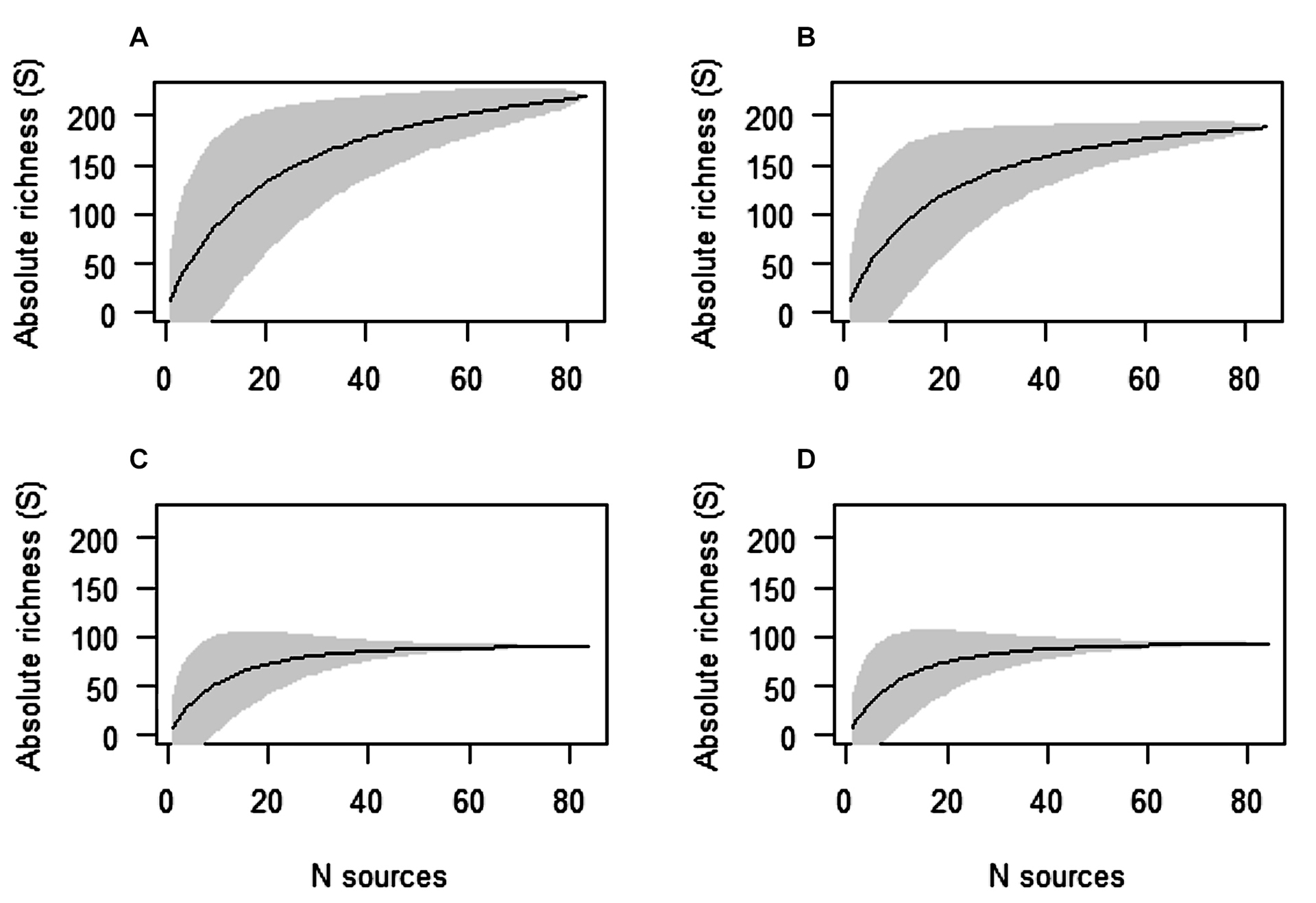
FIGURE 2 | Rarefaction curves for Guanabara Bay’s ichthyofauna richness, Rio de Janeiro, Brazil. A. For the bay as a whole, and for the estuary compartments separately: B. Lower estuary, C. Middle estuary and D. Upper estuary.

FIGURE 3 | Ichthyofauna rates found for Guanabara Bay, Rio de Janeiro, Brazil. A. As a whole and for the B. Lower, C. Middle, and D. Upper estuaries separately, where “mg” corresponds to the number of extra samples needed to reach a “g” for estimated richness. When the line touches the x axis (mg = 0), the “g” values are reached by our study, that is, the value in which extra collections are not necessary.
TABLE 4 | Chao2 parametric estimator values for Guanabara Bay, Rio de Janeiro, Brazil, as a whole, and for the lower, middle and upper estuaries separately (t = 84).
t | T | S obs | S est | Q1 | Q2 | q0 | m | mg | mg | mg | mg | |
Guanabara Bay | 84 | 1054 | 218 | 247.66 | 49 | 40 | 0.046 | 318.96 | 44.83 | 9.25 | – | – |
Lower estuary | 84 | 1005 | 188 | 202.87 | 31 | 32 | 0.031 | 223.52 | 15.49 | – | – | – |
Middle estuary | 84 | 720 | 90 | 90.89 | 3 | 5 | 0.004 | 60.45 | – | – | – | – |
Upper estuary | 84 | 735 | 92 | 92.64 | 3 | 7 | 0.004 | 41.15 | – | – | – | – |
Contrary to the lower estuary compartment and the Guanabara Bay as a whole, stabilization of the rarefaction curves was obtained for the middle and upper estuary compartments (Figs. 2C, D), indicating that the records are sufficient to represent the species richness of these two portions of the bay. The observed and estimated richness values were very close in both cases and q0 values were less than 0.01 (Tab. 4). Even though the “m” values were not null, they indicated a sampling of over 99% for these two compartments (Figs. 3C, D). However, a new species was recorded in the upper estuary after 2020. On June 22, 2022, gillnet artisanal fisherman captured one specimen of the tiger-shark Galeocerdo cuvier on quadrant C4. This is the first record of the species in Guanabara Bay. The specimen was a juvenile female with total length of 1,80 m and its jaw is deposited in the MNRJ (MNRJ 53604).
Spatial distribution. In general, the region of the bay closer to the mouth of the estuary presented the highest values of both absolute richness (S) and species density (SD). Quadrants D7 and E7 at the entrance of the estuary were the richest and densest (Figs. 1, 4). Although D7 presented the highest number of species (127), E7 has the highest density due to its smaller water surface area. High S and SD values were also noted in the other lower estuary quadrants, with D4 having the lowest richness (43 species). However, D6 results were lower than expected (S = 55, SD = 2.34 sp./km2) considering it is a transition region between D7 and D5, both of which are richer.

FIGURE 4 | Distribution of absolute richness (A) and species density (B) per km2 at Guanabara Bay, Rio de Janeiro, Brazil.
A high variation in S was observed in the middle estuary compartment. For instance, quadrants F4 and F5 presented less than 10 species, while quadrants C5 and E5 had over 60 species (Figs. 1, 4A). However, the quadrants of this compartment have very different water surface areas, making SD a more reliable measure for comparison. Even though quadrants B5, F5 and E6 have relatively small S values (18, 2 and 14, respectively), their small water surface area result in SD values above three (Figs. 1, 4B). Therefore, only quadrants C6 and F4 stand out with relativity lower densities when compared to the other quadrants of the middle estuary.
The upper estuary presented most quadrants with relatively lower values of S, with three quadrants with less than 10 species (D2, D3 and E2) and five with less than 20 species (B3, B4, C4, F2 and F3). A similar pattern was recovered for species density, with the upper estuary comprising the only portion of the bay with quadrants with SD values lower than one species per km2 (B4, D3, E2, F2 and F3). All quadrants in the upper estuary compartment, except for C3 and E3, presented SD values lower than two species per km2. Indeed, quadrants C3 (S = 62, SD = 2.98 sp./km2) and E3 (S = 73, SD = 3.07 sp./km2) stood out in terms of richness, with S and SD values more similar to the ones recovered for the lower and middle estuary compartments (Figs. 1, 4).
Temporal changes. From the 220 species considered, 84 were not recorded in the last decade (between 2010 and 2020) (Tab. 5). Among these, 65 species were last recorded between 2000 and 2009, comprising 60 teleosts and five elasmobranchs. However, three of these elasmobranchs (Sphyrna tiburo (Linnaeus, 1758), S. zygaena (Linnaeus, 1758), and Pristis pristis (Linnaeus, 1758)) may have been recorded a long time before this timeframe. That is because their records come from past literature and ichthyological collections data presented at Buckup et al. (2000) who did not present the years that the records were made. Therefore, we considered the year of publication (2000) as the record data of those species.
TABLE 5 | Species not recorded after 2010 at Guanabara Bay, Rio de Janeiro, Brazil, until 2020.
Species last recorded | Dates |
Species last recorded
from 2000 to 2009 | |
Abudefduf saxatilis (Linnaeus, 1758) | 2001 |
Acanthostracion quadricornis (Linnaeus, 1758) | 2005–2007 |
Aluterus heudelotii Hollard, 1855 | 2005–2007 |
Aluterus schoepfii (Walbaum, 1792) | 2005–2007 |
Anchoa marinii Hildebrand, 1943 | 2005–2007 |
Anisotremus virginicus (Linnaeus, 1758) | 2005–2007 |
Antennarius striatus (Shaw,
1794) | 2005–2007 |
Astroscopus y-graecum (Cuvier, 1829) | 1998/2005/2006 |
Bagre bagre (Linnaeus,
1766) | 2005 |
Bairdiella goeldi Marceniuk, Molina, Caires, Rotundo, Wosiacki & Oliveira, 2019 | 1994/2005–2007 |
Bathygobius soporator (Valenciennes, 1837) | 1944/1961/2005–2007 |
Boridia grossidens Cuvier, 1830 | 2005–2007 |
Bothus robinsi Topp & Hoff, 1972 | 2005–2007 |
Bryx dunckeri (Metzelaar, 1919) | 2005/2006 |
Cantherhines pullus (Ranzani,
1842) | 2005/2006 |
Species last recorded
from 2000 to 2009 | |
Canthidermis sufflamen (Mitchill, 1815) | 2005/2006 |
Canthigaster figueiredoi Moura &
Castro, 2002 | 2005/2006 |
Caranx bartholomaei Cuvier, 1833 | 2005/2006 |
Cathorops spixii (Agassiz,
1829) | 1944/2005–2007 |
Conodon nobilis (Linnaeus, 1758) | 2005–2007 |
Cosmocampus elucens (Poey, 1868) | 2005/2006 |
Dactyloscopus crossotus Starks, 1913 | 2005/2006 |
Engraulis anchoita Hubbs & Marini, 1935 | 1977/2005–2007 |
Epinephelus itajara (Lichtenstein, 1822) | 2000/2005/2006 |
Epinephelus morio (Valenciennes,
1828) | 1944/2005/2006 |
Eucinostomus lefroyi (Goode, 1874) | 1998/2005/2006 |
Fistularia
tabacaria Linnaeus, 1758 | 1989/2005–2007 |
Fistularia petimba Lacepède, 1803 | 2005–2007 |
Genyatremus cavifrions (Cuvier, 1830) | 2005/2006 |
Gymnothorax ocellatus Agassiz, 1831 | 1889/1985/2005–2007 |
Haemulopsis corvinaeformis (Steindachner, 1868) | 1993/2005–2007 |
Hemicaranx amblyrhynchus (Cuvier, 1833) | 2005/2006 |
Hippocampus erectus Perry, 1810 | 1953/2000 |
Hippocampus reidi Ginsburg,
1933 | 1989/2000/2005–2007 |
Holocentrus adscensionis (Osbeck, 1765) | 2007 |
Hyporthodus nigritus (Holbrook,
1855) | 2005–2007 |
Hyporthodus niveatus (Valenciennes, 1828) | 2005–2007 |
Lagocephalus lagocephalus (Linnaeus, 1758) | 2005/2006 |
Lepidopus caudatus (Euphrasen, 1788) | 2008 |
Macrodon atricauda (Günther, 1880) | 2001/2002 |
Mullus argentinae Hubbs & Marini, 1933 | 1913/2005–2007 |
Mycteroperca microlepis (Goode & Bean, 1879) | 2005–2007 |
Nebris microps Cuvier, 1830 | 2005–2007 |
Notarius grandicassis (Valenciennes, 1840) | 2005–2007 |
Odontognathus mucronatus Lacepède, 1800 | 2005–2007 |
Pagrus pagrus (Linnaeus,
1758) | 2008/2009 |
Paralichthys orbignyanus (Valenciennes, 1839) | 2005–2007 |
Paralichthys patagonicus Jordan,
1889 | 2005–2007 |
Polydactylus oligodon (Günther, 1860) | 2005/2006 |
Pristis pristis (Linnaeus, 1758) | 2000 |
Pseudobatos horkelii (Müller & Henle, 1841) | 2005–2007 |
Species last recorded
from 2000 to 2009 | |
Pseudobatos percellens (Walbaum, 1792) | 2005–2007 |
Rachycentron canadum (Linnaeus, 1766) | 2005/2006 |
Scartella cristata (Linnaeus, 1758) | 1982/1995/2005/2006 |
Scorpaena plumieri Bloch,
1789 | 1989/2005–2007 |
Sphyrna zygaena (Linnaeus, 1758) | 2000 |
Sphyrna tiburo (Linnaeus,
1758) | 2000 |
Stellifer brasiliensis (Schultz, 1945) | 2005–2007 |
Strongylura marina (Walbaum, 1792) | 2005–2007 |
Syacium micrurum Ranzani, 1842 | 2005–2007 |
Syacium papillosum (Linnaeus, 1758) | 2005–2007 |
Syngnathus pelagicus Linnaeus, 1758 | 1960/1989/2005/2006 |
Trachinocephalus myops (Forster,
1801) | 2005–2007 |
Trachurus lathami Nichols, 1920 | 2005–2007 |
Species last recorded
from 1990 to 1999 | |
Tomicodon australis Briggs, 1955 | 1999 |
Epinephelus marginatus (Lowe, 1834) | 1913/1956/1991/1997 |
Rhinoptera bonasus (Mitchill, 1815) | 1997 |
Rhizoprionodon lalandii (Valenciennes, 1839) | 1997 |
Rhizoprionodon porosus (Poey, 1861) | 1997 |
Serranus flaviventris (Cuvier, 1829) | 1944/1992/1997 |
Species last recorded
from 1980 to 1989 | |
Diapterus auratus Ranzani, 1842 | 1944/1989 |
Gobiesox barbatulus (Starks, 1913) | 1955/1989 |
Hyporhamphus unifasciatus (Ranzani, 1841) | 1944/1989 |
Species last recorded
from 1960 to 1969 | |
Hypleurochilus fissicornis (Quoy & Gaimard, 1824) | 1961 |
Myrichthys ocellatus (Lesueur, 1825) | 1964 |
Remora remora (Linnaeus,
1758) | 1961 |
Symphurus plagusia (Bloch
& Schneider, 1801) | 1968 |
Species last recorded
from 1950 to 1959 | |
Microgobius carri Fowler, 1945 | 1955 |
Aetobatus narinari (Euphrasen, 1790) | 1957 |
Diodon hystrix Linnaeus, 1758 | 1954/1956 |
Species last recorded
from 1940 to 1949 | |
Mugil curvidens Valenciennes, 1836 | 1944 |
Species last recorded
from 1930 to 1939 | |
Narcine brasiliensis (Olfers, 1831) | 1938 |
Species last recorded
from 1910 to 1919 | |
Parablennius pilicornis (Cuvier, 1829) | 1915 |
Six species, three teleosts and three elasmobranchs (Tab. 5), were last recorded in Guanabara Bay between 1990 and 1999. The teleost Tomicodon australis Briggs, 1955, the sharks Rhizoprionodon lalandii and R. porosus (Poey, 1861) and the ray Rhinoptera bonasus (Mitchill, 1815) are represented by only one record each in the MNRJ Fish Collection, while the teleosts Epinephelus marginatus (Lowe, 1834) and Serranus flaviventris (Cuvier, 1829) were recorded at different dates until 1997, when both species ceased to appear in the records. The most recent records for the teleosts Hyporhamphus unifasciatus (Ranzani, 1841), Diapterus auratus Ranzani, 1842, and Gobiesox barbatulus (Starks, 1913) were all made in 1989.
Four species were recorded between 1960 and 1969 and three others were mentioned only between 1960 and 1969 (Tab. 5). Last records of some species are considerably older, for instance Mugil curvidens Valenciennes, 1836, recorded in 1944, Narcine brasiliensis (Olfers, 1831), in 1938, and Parablennius pilicornis (Cuvier, 1829), in 1915. Data of those records are again based on voucher specimens at MNRJ.
Nevertheless, fishing landing monitoring is still being carried out at Guanabara Bay, resulting in new records. After 2020, two new records of species shown on Tab. 5 were registered. On August 9, 2022, a 30 cm (total length) female Rhizoprionodon lalandii was captured by fishing at quadrant D2 and was deposited at MNRJ (MNRJ 53605). The species was recorded at the bay only once before in 1997. The other species is the teleost Bagre bagre previously recorded in 2005. The new record occurred on November 3, 2022, at quadrant F2.
Discussion
The use of different sources for the compilation of past data was an efficient way to build a baseline of fish species from Guanabara Bay, as the different sources filled different gaps regarding the ichthyofauna survey. While the published literature provided more recent records, specimens deposited in ichthyological collections revealed more ancient occurrences, some dating back to the 19th century. Scientific sampling and taxonomic monitoring of fish landings, in turn, revealed 13 species not reported by any other type of source. Since this survey is based on past records, it is important to consider the possibility of misidentification of specimens in the sources consulted. For the scientific sampling and fish landings monitoring this problem was likely minimized, since they were carried out by BioTecPesca/UFRJ and all specimens were identified by a specialist. The use of only published data also increases the reliability of the baseline, since all the articles used were peer reviewed by specialists. Other important measure was the exclusion of doubtful records of species that are not confirmed to occur in the state of Rio de Janeiro. Finally, our survey recovered a considerable level of internal data consistency, with the same species recorded in the same areas by different sources, increasing the reliability of the occurrence of these species.
The total richness of 220 species (203 teleosts and 17 elasmobranchs) recorded was higher than previously reported for the Guanabara Bay. Vianna et al. (2012), for instance, reported 174 species (169 teleosts and five elasmobranchs). Even though this increase in richness was influenced by the new studies published and the new scientific samplings and fishery landing monitoring since 2012, the inclusion of historical records from scientific collections also contributed substantially. Regarding elasmobranchs, for example, Dasyatis hypostigma Santos & Carvalho, 2004, Gymnura altavela (Linnaeus, 1758), Hypanus guttatus (Bloch & Schneider, 1801), Pseudobatos horkelii (Müller & Henle, 1841), Pseudobatos percellens (Walbaum, 1792), and Zapteryx brevirostris (Müller & Henle, 1841) were recorded between 2012 and 2015 (Gonçalves-Silva, Vianna, 2018a), while Carcharhinus brachyurus (Günther, 1870), Rhizoprionodon lalandii, R. porosus, Aetobatus narinari (Euphrasen, 1790), Rhinoptera bonasus, and Narcine brasiliensis were only found as vouchers deposited in collections.
Despite advances, some taxonomic questions still hinder the establishment of a more comprehensive list of fish species in the Guanabara Bay. For instance, Elops saurus Linnaeus, 1766was considered the only species of the genus Elops in the western Atlantic before the description of Elops smithi McBride, Rocha, Ruiz-Carus & Bowen,2010. However, the two species are anatomically similar, such that sympatry of the two species in the region cannot be ruled out at the moment. A similar situation refers to the distribution of Scomber japonicus Houttuyn, 1782. Fricke et al. (2023) indicates that its distribution is restricted to the Pacific Ocean. However, other studies have recognized S. japonicus as occurring in the southwestern Atlantic (Roldán et al., 2000; Perrotta et al., 2005) and specifically of Rio de Janeiro State (Alves et al., 2003; Menezes et al., 2003). Further studies are required to clarify the distribution of those species.
The total species richness recorded in the Guanabara Bay is considerably higher in relation to other tropical estuaries (Tab. 6). The coast of the state of Rio de Janeiro is the richest portion in the Brazilian coast concerning estuarine fish species (Vilar et al., 2017), and Guanabara Bay stands out when compared to two other estuaries previously inventoried in the state (Sepetiba Bay and Mambucaba Estuary), having practically twice the number of species. Even though the large size of the Guanabara Bay contributes to a naturally greater richness, this factor alone is not able to explain the observed discrepancies. Sepetiba Bay, for instance, is similar in size to Guanabara Bay, but has practically half the number of species. Other example is the Bay of Malaga, in Colombia, that despite being much smaller (126 km2) still presents three families, 36 genera and 17 species more than what we recorded at Guanabara Bay.
TABLE 6 | Absolute ichthyofauna richness in tropical estuaries in Brazil and worldwide according to the available literature.
Estuary | Locality | Families | Genera | Species | Area (km2) | References |
Guanabara Bay | Brazil, southeast | 72 | 149 | 220 | 384 | This study |
Sepetiba Bay | Brazil, southeast | 44 | 80 | 107 | 305 | Araújo et al. (2002) |
Mambucaba estuary | Brazil, southeast | 40 | 81 | 111 | 3.82 | Neves et al. (2011) |
Pinheiros Bay | Brazil, south | 29 | 49 | 61 | 200 | Pichler et al. (2015) |
Saco da Fazenda
| Brazil, south | 21 | 35 | 42 | 0.7 | Barreiros et al. (2009) |
São Caetano de
Odivelas e Vigia | Brazil, north | 23 | 46 | 58 | 13.4 | Barros et al. (2011) |
Caeté River estuary | Brazil, north | 82 | 67 | 29 | 93.2 | Barletta et al. (2005) |
Paraguaçu River
estuary | Brazil, northeast | 49 | 83 | 124 | 128 | Reis-Filho et al. (2010) |
Formoso River estuary | Brazil, northeast | 39 | 59 | 78 | 27 | Paiva et al. (2009) |
Mataripe River estuary | Brazil, northeast | 15 | 29 | 35 | 18.5 | Dias et al. (2011) |
Mamanguape | Brazil, northeast | 23 | 31 | 37 | 6.9 | Xavier et al. (2012) |
Buenaventura Bay | Colombia, west | 29 | – | 69 | 70 | Molina et al. (2020) |
Málaga Bay | Colombia, west | 75 | 185 | 237 | 126 | Castellanos-Galindo et al. (2006) |
Sabancuy estuary | Mexico, Yucatán Peninsula | 21 | 27 | 33 | 8.71 | González-Solis, Torruco
(2013) |
Embley estuary | Australia, north | – | – | 197 | 75 | Blaber et al. (1989) |
Vellar estuary | India, southeast | 42 | 61 | 95 | 2.62 | Murugan et al. (2014) |
Zuari | India, west | – | – | 176 | 39.9 | Sreekanth et al. (2020) |
Mandovi | India, west | – | – | 154 | 35.5 | Sreekanth et al. (2020) |
Terekhol | India, west | – | – | 131 | 12.7 | Sreekanth et al. (2020) |
Kali | India, west | – | – | 133 | 20.8 | Sreekanth et al. (2020) |
Gâmbia estuary | Gâmbia | 32 | 54 | 70 | 624 | Albaret et al. (2004) |
Morrumbene | Mozambique, east | – | 84 | 114 | 193 | Day (1974) |
The relatively high value of species richness in the Guanabara Bay is likely promoted by the diversity of environments and microhabitats, as the bay encompasses islands, mangroves, rocky shores, sandy beaches, artificial substates and muddy bottoms. In addition, the bay presents a wide variation of environmental conditions and gradients of salinity and nutrient distribution that are characteristic of estuaries (Vianna et al., 2012; Silva-Junior et al., 2016; Wolanski, Elliott, 2016). These conditions promote a wide variety of ecological opportunities, reducing competition and favoring the coexistence of a high number of species (Bello et al., 2012; Dolbeth et al., 2016). Furthermore, the bay conditions are seasonally influenced by a low intensity upwelling event. During spring and summer (November to March) changes in winds promote the outcrop of cold waters from the SACW mass, causing parts of the estuary to present subtropical temperatures (between 10 and 20 ºC) (Silva-Junior et al., 2016). This phenomenon allows species that only occur in deeper areas of the continental shelf to enter the estuary.
Concerning the absolute richness accumulation curves calculated, the upper and middle estuary curves stabilized, indicating that richness values recorded are close to the estimated value of those compartments. However, the record of Galeocerdo cuvier made in the upper estuary compartment in 2022 indicates that occasional species may occur even in the inner parts of the bay, especially when it comes to opportunistic highly mobile taxa.
Stabilization of the accumulation curves were not observed for the Guanabara Bay as a whole and for the lower estuary, both of which are likely to have larger values of richness than the ones recorded here. The lower estuary seems to have strongly influenced this result. Sampling effort required to reach an asymptote can be prohibitively large for environments with a high number of rare species (Chao et al., 2009). As the region closest to the adjacent coastal zone, the lower estuary is affected by the continuous inflow of oceanic water and is visited by many occasional opportunistic marine species, which functionally act as rare species. For instance, species associated with rocky shores from some beaches around the Guanabara Bay (e.g., Rodrigues-Barreto et al., 2017) probably enter the estuary during tide variations. However, their record can be hampered by the high turbidity that hinders visual census attempts. Indeed, the Chao2 index calculated unusually high “m” values for the lower estuary, indicating that approximately 223 new sources would be needed for the entire ichthyofauna to be inventoried in that compartment. Therefore, the non-stabilization of the lower estuary compartment may be preventing the stabilization of the Guanabara Bay’s richness accumulation curve. This is a common situation in tropical environments, where different ecosystems have been sampled for decades without reaching an asymptote in the species richness (e.g., Gotelli, Colwell, 2011).
The distribution of the estuarine ichthyofauna is influenced by the interaction between coastal currents and the water from the local drainage basin, as well as by the degree of tolerance of each species to the salinity gradient (Camargo, Issac, 2003; Silva-Junior et al., 2016). Other important factors are the colonization capacity of different fish populations and the variety of habitats and biotic interactions that maximize interspecific coexistence (Bello et al., 2012; Dolbeth et al., 2016). The lower estuary is the compartment of the bay most influenced by coastal oceanic waters, allowing marine species to enter the compartment to feed (Nybakken, Bertness, 2005). These occasional marine species are likely to promote the high S and SD values in the lower estuary. The proximity to the coastal environments seems to produce a gradient in this compartment, with the innermost quadrants (D4 and E4) presenting lower values of S and SD than the outmost quadrants (D5, D7 and E7) (Fig. 1). The only quadrant that deviates from this pattern is D6. However, this is probably due to the difficulty of performing biological samplings, since this quadrant presents depths up to 50 m (Meniconi et al., 2012) and undergoes intense boat traffic.
The middle estuary is a transition area, presenting distinct spatial and temporal features. This compartment can be split into two portions that respond differently to the dry and rainy seasons, namely (A) the quadrants to the left of the central channel (B5, C5 and C6) and (B) the quadrants to the right of the central channel (E5, E6, F4 and F5) (Fig. 1). In general, the water column conditions during the rainy season are more variable than in the dry season, but in A the greatest amplitudes are related to temperature (minimum of 17 ºC and maximum of 28 ºC), while in B salinity is more variable (minimum of 18.8 S and maximum of 33.6) (Silva-Junior et al., 2016). The SD value of quadrant C6 differs from the rest of the quadrants of A, being the only one with SD lower than 3.0. As salinity does not vary considerably within this group, this low value is probably related to the fact that this location has been the subject of few studies and is not a BioTecPesca collection point, resulting in a lower sampling of this quadrant. In B, the F4 quadrant presented SD values lower than the rest (1.63 sp/km2). In this case, lower SD values are probably caused by both a methodological factor (all records come from source 63) and to the innermost position of this quadrant, which makes it difficult for species that do not support lower salinities to inhabit.
Lower salinities may also play a role on the low S and SD values recorded in the upper estuary compartment, preventing marine coastal species from accessing the innermost part of the bay (Nybakken, Bertness, 2005; Silva-Junior et al., 2016; Souza, Vianna, 2022). Another important factor is that the upper estuary is the most environmentally impacted portion of the bay. In addition to receiving pollutants from rivers (e.g., untreated sewage and inorganic pollutants), natural water renewal is slow, resulting in low environmental quality anoxic zones. (Fistarol et al., 2015). However, two quadrants (E3 and C3) stood out with much higher S and SD values than the rest of the upper estuary. The absolute richness of 73 species found in E3 may be a result of the influence of the central channel during drought periods, when more saline waters advance to more inland estuarine regions, and the wide variety of habitats associated with the Paquetá island located in that region. Quadrant C3, on the other hand, is relatively far from the central channel and has no islands. The high S and SD values of C3 are thereby more likely to be related to collection efforts, as C3 was a BioTecPesca collection point. It also might be noteworthy that, both quadrants with higher S and SD values are within the influence of Protected Areas (Fig. 1). Quadrant E3 is very close to the APA Guapimirim, while the Barão de Mauá Municipal Natural Park is located on C3’s coast. These Protected Areas may be relieving local anthropic impacts such as over-fishing, allowing for a higher number of species to be recorded in its vicinities.
Our results also suggest that temporal changes in the composition of Guanabara Bay’s ichthyofauna occurred over the decades. As much as the absence of records between 2010 and 2020 is indicative of local extinction or at least of abundance reduction of species, more studies are still required to confirm this situation as shown by the recent records of Rhizoprionodon lalandii and Bagre bagre in 2022. Among the 84 species unrecorded from 2010 to 2020 (Tab. 5), 81% are not estuarine-dependent. Thus, the lack of more recent records for this non-dependent species may be due to their non-obligatory relation with the estuary coupled with declining environmental conditions. Another factor to be considered is the habitat of those species since there is a lack of recent studies in more consolidated substrate regions in the interior of the bay.
The decreased sampling efforts by BioTecPesca is especially important when it comes to the species last recorded between 1990 and 2010. The main sampling method used by BioTecPesca was bottom trawling, which results mostly in the capture of demersal species of unconsolidated substrate. Therefore, pelagic species like Hemicaranx amblyrhynchus (Cuvier, 1833), Rhinoptera bonasus, Rhizoprionodon lalandii, R. porosus,and Syngnathus pelagicus Linnaeus, 1758 would not be easily captured, so that their local extinction cannot be attested. This hypothesis is again supported by the new record of R. lalandii since this species was previously only recorded in 1997 but was captured by fisherman in 2022. Furthermore, collections made by BioTecPesca in 2013 and 2014 were less numerous and covered fewer locations when compared to the period between 2005 to 2007, thus hampering more recent records of species that do not commonly appear in scientific papers and are not recorded in fishing landings.
However, of the 70 species last recorded between 1990 and 2010, six are at risk of extinction at the global level (Mycteroperca microlepis (Goode & Bean, 1879), Paralichthys patagonicus Jordan, 1889, Pseudobatos percellens, Rhinoptera bonasus, Rhizoprionodon lalandii,and R. porosus), two are threatened at the national level (Hippocampus reidi Ginsburg, 1933 and Hyporthodus nigritus (Holbrook, 1855)) and nine are threatened at both levels (Epinephelus itajara (Lichtenstein, 1822), E. marginatus, E. morio (Valenciennes, 1828), Hippocampus erectus Perry, 1810, Hyporthodus niveatus (Valenciennes, 1828), Pristis pristis, Pseudobatos horkelii, Sphyrna zygaena, and S. tiburo). For those species, abundance reduction at some level is likely to have occurred at Guanabara Bay. Considering the large number of studies and collections carried out after 1990, local extinction or great abundance reduction are also very likely to have occurred for the 13 species last recorded before 1990. These species span a wide functional range including pelagic and demersal species which are dependent or not dependent on the estuary.
Another worrying result recovered in this survey is that of the 17 elasmobranchs species, 10 (58.8%) were not recorded between 2010 and 2020. A well-documented case of elasmobranch regional extinction is the sawfish Pristis pristis, formerly occurring from northern Brazil to São Paulo and now restricted to the northern regions of Brazil (Fernandez-Carvalho et al., 2013). The disappearance of high trophic level predators is of concern for biodiversity conservation, as these animals play an important role in the ecosystem regulating prey populations. Besides, estuaries are extremely important for sharks and rays, serving both as a feeding area and as nursery grounds (Gonçalves-Silva, Vianna, 2018a; Plumlee et al., 2018). Signs of population reduction for these species in a large estuary such as Guanabara Bay may indicate the decline of elasmobranch populations throughout southeastern Brazil.
Even though Guanabara Bay still has a relatively rich ichthyofauna, with wide taxonomic and functional fish diversity, the implementation of management and conservation actions are paramount to reduce the loss of the biological richness recorded in our study in the more recent decades. There is a need for improvement of the environmental quality of the bay and adjacent regions. Many urban centers around the bay still dump untreated sewage in the estuary (Elk et al., 2022), and therefore it is necessary to expand the sewage collection network that leads the waste to sewage treatment centers. Other important action is the promotion of fisheries management measures focused on sustainable practices. We recommend the prohibition of bottom trawling at Guanabara Bay, since it is an extremely impactful fishing technique that is already forbidden in many Brazilian estuaries. Lastly, our results highlighted the potential of Protected Areas to promote fish species conservation. Our results indicate that Guanabara Bay would benefit largely from the establishment of new protected areas aimed to preserve mangrove ecosystems in its area. Mangroves serve as nursery grounds for many fish species, including highly threatened elasmobranchs, hence reforestation efforts would improve species recovery and promote the conservation of the bay’s ichthyofauna.
Acknowledgments
This study was supported by the Long-Term Ecological Program “Environmental Assessment of Guanabara Bay” – CNPq (PELD 403809/2012–6) and FAPERJ (E26/110.114/2013 and E26/112.636/2012). We thank our colleagues at BioTecPesca (UFRJ) and Guanabara Bay fishers for their help throughout the work. Special thanks are due to Fabio Di Dario (NUPEM/UFRJ), Erica P. Caramaschi (IB/UFRJ), Jean L. Valentin (IB/UFRJ), Sergio Santos (BioTecPesca/UFRJ), and Gabriel B. G. Souza (BioTecPesca/UFRJ) for offering their thoughts on the present study, and to Alfredo Carvalho Filho for reviewing the list of species that compose this baseline.
References
Albaret J-J, Simier M, Darboe FS, Ecoutin J-M, Raffray J, Morais LT. Fish diversity and distribution in the Gambia Estuary, West Africa, in relation to environmental variables. Aquat Living Resour. 2004; 17(1):35–46. https://doi.org/10.1051/alr:2004001
Alves DR, Luque JL, Abdallah VD. Metazoan parasites of chub mackerel, Scomber japonicus (Osteichthyes: Scombridae), from the coastal zone of the State of Rio de Janeiro, Brazil. Rev Bras Parasitol Vet. 2003; 12(4):164–70. Available from: http://www.ufrrj.br/laboratorio/parasitologia/arquivos/publicacao/56_LIVRO.pdf
Andrade AC, Santos SR, Verani JR, Vianna M. Guild composition and habitat use by Tetraodontiformes (Teleostei, Acanthopterygii) in a south-western Atlantic tropical estuary. J Mar Biol Assoc United Kingdom. 2016; 96(6):1251–64. https://doi.org/10.1017/S0025315415001368
Andrade-Tubino MF, Ribeiro ALR, Vianna M. Organização espaço-temporal das ictiocenoses demersais nos ecossistemas estuarinos brasileiros: uma síntese. Oecologia Aust. 2008; 12(4):640–61. https://doi.org/10.4257/oeco.2008.1204.05
Araújo FG, Azevedo MCC, Silva MA, Pessanha ALM, Gomes ID, Cruz-Filho AG. Environmental influences on the demersal fish assemblages in the Sepetiba Bay, Brazil. Estuar Res Fed. 2002; 25(3):441–50.
Baêta AP, Kehrig HA, Malm O, Moreira I. Total mercury and methylmercury in fish from a tropical estuary. Environ Toxicol. 2006; 10:183–92. https://doi.org/10.2495/ETOX060181
Barletta M, Barletta-Bergan A, Saint-Paul U, Hubold G. The role of salinity in structuring the fish assemblages in a tropical estuary. J Fish Biol. 2005; 66(1):45–72. https://doi.org/10.1111/j.0022-1112.2005.00582.x
Barreiros JP, Branco JO, Freitas Jr. F, Machado L, Hostim-Silva M, Verani JR. Space–time distribution of the ichthyofauna from Saco da Fazenda estuary, Itajaí, Santa Catarina, Brazil. J Coast Res. 2009; 25(5):1114–21. https://doi.org/10.2112/08-1050.1
Barros DF, Torres MF, Frédou FL. Ictiofauna do estuário de São Caetano de Odivelas e Vigia (Pará, Estuário Amazônico). Biota Neotrop. 2011; 11(2):387–72. https://doi.org/10.1590/S1676-06032011000200035
Bello F, Price JN, Münkemüller T, Liira J, Zobel M, Thuiller W et al. Functional species pool framework to test for biotic effects on community assembly. Ecol Soc Am. 2012; 93(10):2263–73. https://doi.org/10.1890/11-1394.1
Blaber SJM, Brewer DT, Salini JP. Species composition and biomasses of fishes in different habitats of a tropical Northern Australian estuary: their occurrence in the adjoining sea and estuarine dependence. Estuar Coast Shelf Sci. 1989; 29(6):509–31. https://doi.org/10.1016/0272-7714(89)90008-5
Brum MJI, Corrêa MMO, Oliveira CC, Galetti Jr. PM. Cytogenetic studies on the Perciformes Orthopristis ruber (Haemulidae) and Scartella cristata (Blenniidae). Caryologia. 1995; 48(3–4):309–18. https://doi.org/10.1080/00087114.1995.10797340
Brum MJI. Cytogenetic studies in tetraodontiforms Sphoeroides tyleri (Tetraodontidae) and Chilomycteras spinasus (Diodontidae) from Rio de Janeiro Coast, Brazil. Chromosome Sci. 2000; 4(3):103–05.
Buckup PA, Nunan GW, Gomes UL, Costa WJEM, Gadig OBF. Peixes. In: Maio FRD, Silva MBR, Araújo TN, editors. Espécies ameaçadas extinção no Municipio do Rio Janeiro. Rio de Janeiro: Prefeitura da Cidade do Rio de Janeiro, Secretaria do Meio Ambiente; 2000. p.52–57.
Camargo M, Issac VJ. Ictiofauna Estuarina. In: Fernandes MEB, editor. Os manguezais da costa norte brasileira. Maranhão: Fundação Rio Bacanga; 2003. p.105–42.
Castellanos-Galindo GA, Caicedo-Pantoja JA, Mejía-Ladino LM, Rubio E. Marine and estuarine fishes of Malaga Bay, Valle del Cauca, colombian Pacific Ocean. Biota Colomb. 2006; 7(2):263–82.
Chao A, Colwell RK, Lin C-W, Gotelli NJ. Sufficient sampling for asymptotic minimum species richness estimators. Ecology. 2009; 90(4):1125–33. https://doi.org/10.1890/07-2147.1
Corrêa B, Vianna M. Spatial and temporal distribution patterns of the silver mojarra Eucinostomus argenteus (Perciformes: Gerreidae) in a tropical semi-enclosed bay. J Fish Biol. 2015; 89(1):641–60. https://doi.org/10.1111/jfb.12843
Day JH. The ecology of Morrumbene estuary, Moçambique. Trans R Soc South Africa. 1974; 41(1):43–97. https://doi.org/10.1080/00359197409519438
Dias JF, Gonçalves AM, Fernandez WS, Silbiger HLN, Fiadi CB, Schmidt TCS. Ichthyofauna in an estuary of the Mataripe area, Todos os Santos Bay, Bahia, Brazil. Brazilian J Oceanogr. 2011; 59(1):75–95. https://doi.org/10.1590/S1679-87592011000100006
Dolbeth M, Vendel AL, Baeta A, Pessanha A, Patrício J. Exploring ecosystem functioning in two Brazilian estuaries integrating fish diversity, species traits and food webs. Mar Ecol Prog Ser. 2016; 560:41–55. https://doi.org/10.3354/meps11895
Elk AGHP, D’Oliveira PMS, Giordano G, Andrade RC. Potencial poluidor da disposição final de resíduos sólidos nas águas da bacia hidrográfica da Baía de Guanabara – RJ. Eng Sanit Ambient. 2022; 27(1):195–203. https://doi.org/10.1590/S1413-415220200319
Elliott M, Whitfield AK, Potter IC, Blaber SJM, Cyrus DP, Nordlie FG et al. The guild approach to categorizing estuarine fish assemblages: A global review. Fish Fish. 2007; 8(3):241–68. https://doi.org/10.1111/j.1467-2679.2007.00253.x
Fernandez-Carvalho J, Imhoff JL, Faria VV, Carlson JK, Burgess GH. Status and the potential for extinction of the largetooth sawfish Pristis pristis in the Atlantic Ocean. Aquat Conserv Mar Freshw Ecosyst. 2013; 24(4):478–97. https://doi.org/10.1002/aqc.2394
Fistarol GO, Coutinho FH, Moreira APB, Venas T, Cánovas A, Paula Jr. SEM et al. Environmental and sanitary conditions of Guanabara Bay, Rio de Janeiro. Front Microbiol. 2015; 6:1–17. https://doi.org/10.3389/fmicb.2015.01232
Fricke R, Eschmeyer WN, Van der Laan R. Eschmeyer’s catalog of fishes: genera, species, references [Internet]. San Francisco: California Academy of Science; 2023. Available from: http://researcharchive.calacademy.org/research/ichthyology/catalog/fishcatmain.asp
Gomes DC, Fabio SP, Rolas FJT. Contribuição para o conhecimento dos parasitos de peixes do litoral do estado da Guanabara – Parte II. Mem Inst Oswaldo Cruz. 1974; 72:9–19. https://doi.org/10.1590/S0074-02761974000100003
Gonçalves-Silva F, Vianna M. Use of a species-rich and degraded tropical estuary by Elasmobranchs. Brazilian J Ocean. 2018a; 66(4):339–46.
Gonçalves-Silva F, Vianna M. Diet and reproductive aspects of the endangered butterfly ray Gymnura altavela raising the discussion of a possible nursery area in a highly impacted environment. Brazilian J Oceanogr. 2018b; 66(3):315–24. https://doi.org/10.1590/s1679-8759201801906603
González-Solis A, Torruco D. Fish assemblage structure in relation to environmental conditions in a tropical estuary. Rev Biol Mar Oceanogr. 2013; 48(3):553–63. https://doi.org/10.4067/S0718-19572013000300012
Gotelli NJ, Colwell RK. Estimating species richness. In: Magurran AE, McGill BJ, editors. Biological Diversity: Frontiers in Measurement and Assessment. Oxford: Oxford University Press; 2011. p.39–54.
Hauser-Davis RA, Lopes RM, Ziolli RL. Inihibition of mullet (M. liza) brain acetylcholinesterase activity by in vitro polycyclic aromatic hydrocarbon exposure. Mar Pollut Bull. 2019; 140:30–34. https://doi.org/10.1016/j.marpolbul.2019.01.027
Hoenig JM, Gruber SH. Life-history patterns in the elasmobranchs: implications for fisheries management. In: Pratt Jr. HL, Gruber SH, Taniuchi T, editors. Elasmobranchs as living resources: advances in the biology, ecology, systematics, and the status of fisheries. Springfield: NOAA Technological Report NMFS 90; 1990, p.1–16.
Menezes NA, Buckup PA, Figueiredo JL, Moura RL. Catálogo das espécies de peixes marinhos do Brasil. São Paulo: Museu de Zoologia USP; 2003.
Meniconi MFG, Silva TA, Fonseca ML, Lima SOF, Lima EFA, Lavrado HP et al. A Baía de Guanabara. In: Meniconi MFG, Silva TA, Fonseca ML, Lima SOF, Lima EFA, Lavrado HP et al., editors. Baía Guanabara Síntese do Conhecimento Ambiental – Biodiversidade. Rio de Janeiro: Petrobras; 2012. p.10–14.
Mérigot B, Frédou FL, Viana AP, Ferreira BP, Nascimento Jr. EC, Beserra Jr. CAS et al. Fish assemblages in tropical estuaries of northeast Brazil: A multi-component diversity approach. Ocean Coast Manag. 2017; 143:175–83. https://doi.org/10.1016/j.ocecoaman.2016.08.004
Molina A, Duque G, Cogua P. Influences of environmental conditions in the fish assemblage structure of a tropical estuary. Mar Biodivers. 2020; 50(5):1–13. https://doi.org/10.1007/s12526-019-01023-0
Mulato IP, Corrêa B, Vianna M. Time-space distribution of Micropogonias furnieri (Perciformes, sciaenidae) in a tropical estuary in southeastern Brazil. Bol Inst Pesca. 2015; 41(1):1–18.
Murugan S, Ajmal-Khan S, Lyla PS, Manokaran S, Raja S, Akabar-John B. Spatial and temporal variability in fish diversity of Vellar estuary (south east coast of India). Annu Res Rev Biol. 2014; 4(13):2147–62. https://doi.org/10.9734/ARRB/2014/4962
Neves LM, Teixeira TP, Araújo FG. Structure and dynamics of distinct fish assemblages in three reaches (upper, middle and lower) of an open tropical estuary in Brazil. Mar Ecol. 2011; 32(1):115–31. https://doi.org/10.1111/j.1439-0485.2010.00407.x
Nybakken JW, Bertness MD. Estuaries and salt marshes. In: Nybakken JW, Bertness MD, editors. Marine Biology an Ecological Approach. San Francisco: Pearson Education, Inc., publishing as Benjamin Cummings; 2005. p.368–71.
Paiva ACG, Lima MFV, Souza JRB, Araújo ME. Spatial distribution of the estuarine ichthyofauna of the rio Formoso (Pernambuco, Brazil), with emphasis on reef fish. Zoologia. 2009; 26(2):266–78. https://doi.org/10.1590/S1984-46702009000200009
Paiva LG, Vannuci-Silva M, Correa B, Santos-Neto E, Vianna M, Lailson-Brito JL. Additional pressure to a threatened species: High persistent organic pollutant concentrations in the tropical estuarine batoid Gymnura altavela. Bull Environ Contam Toxicol. 2021; 107(1):37–44. https://doi.org/10.1007/s00128-021-03151-5
Pereira E, Baptista-Neto JA, Smith BJ, Mcallister JJ. The contribution of heavy metal pollution derived from highway runoff to Guanabara Bay sediments: Rio de Janeiro/Brazil. An Acad Bras Cienc. 2007; 79(4):739–50. https://doi.org/10.1590/S0001-37652007000400013
Perrotta RG, Carvalho N, Isidro E. Comparative study on growth of chub mackerel (Scomber japonicus Houttuyn, 1782) from three different regions: NW Mediterranean, NE and SW Atlantic. Rev Invest Desarr Pesq. 2005; 17:67–79. Available from: https://aquadocs.org/handle/1834/1562
Pichler HA, Spach HL, Gray CA, Broadhurst MK, Schwarz R, Oliveira-Neto JF. Environmental influences on resident and transient fishes across shallow estuarine beaches and tidal flats in a Brazilian World Heritage area. Estuar Coast Shelf Sci. 2015; 164:482–92. https://doi.org/10.1016/j.ecss.2015.07.041
Plumlee JD, Dance KM, Matich P, Mohan JA, Richards TM, TinHan TC et al. Community structure of elasmobranchs in estuaries along the northwest Gulf of Mexico. Estuar Coast Shelf Sci. 2018; 204:103–13. https://doi.org/10.1016/j.ecss.2018.02.023
Pratt Jr. HL, Gruber SH, Taniuchi T. Elasmobranchs as living resources: advances in the biology, ecology, systematics, and the status of fisheries. Springfield: NOAA Technological Report NMFS 90; 1990.
Prestrelo L, Vianna M. Identifying multiple-use conflicts prior to marine spatial planning: A case study of a multi-legislative estuary in Brazil. Mar Policy. 2016; 67:83–93. https://doi.org/10.1016/j.marpol.2016.02.001
Reis-Filho JA, Nunes JACC, Ferreira A. Estuarine ichthyofauna of the Paraguaçu River, Todos os Santos Bay, Bahia, Brazil. Biota Neotrop. 2010; 10(4):301–11. https://doi.org/10.1590/S1676-06032010000400034
Rodrigues-Barreto N, Shimada-Brotto DV, Guterres-Giordano R, Andrade-Bertoncino A, Santos LN. The rocky reef fishes of Vermelha Beach, a marine-estuarine transitional zone at Guanabara Bay, Brazil. Lat Am J Aquat. 2017; 45(1):33–40. https://doi.org/10.3856/vol45-issue1-fulltext-4
Roldán MI, Perrotta RG, Cortey M, Pla C. Molecular and morphologic approches to discrimination of variability patters in chub mackerel, Scomber japonicus. J Exp Mar Biol Ecol. 2000; 253(1):63–74. https://doi.org/10.1016/S0022-0981(00)00244-6
Rosenfelder N, Lehnert K, Kaffarnik S, Torres JPM, Vianna M, Vetter W. Thorough analysis of polyhalogenated compounds in ray liver samples off the coast of Rio de Janeiro, Brazil. Environ Sci Pollut Res. 2012; 19(2):379–89. https://doi.org/10.1007/s11356-011-0569-2
Santos SR, Andrade AC, Verani JR, Vianna M. Population explosion of the burrfish Chilomycterus spinosus spinosus (Diodontidae, Tetraodontiformes) in a eutrophic tropical estuary. Mar Biol Res. 2015; 11(9):955–64. https://doi.org/10.1080/17451000.2015.1045000
Santos SR, Galvão KP, Adler GH, Andrade-Tubino MF, Vianna M. Spatiotemporal distribution and population biology aspects of Cetengraulis edentulus (Actinopterygii: Clupeiformes: Engraulidae) in a south-western atlantic estuary, with notes on the local Clupeiformes community: conservation implications. Acta Ichthyol Piscat. 2020; 50(2):139–50. https://doi.org/10.3750/AIEP/02511
Schilling AC, Batista JLF, Couto HZ. Ausência de estabilização da curva de acumulação de espécies em florestras tropicais. Ciência Florest. 2012; 22(1):101–11.
Sheaves M. Scale-dependent variation in composition of fish fauna among sandy tropical estuarine embayments. Mar Ecol Prog Ser. 2006; 310:173–84. https://doi.org/10.3354/meps310173
Silva-Junior DR, Gomes VS, Linde-Arias AR, Vianna M. Metallothionein in the pond perch Diplectrum radiale (Teleostei) as a biomarker of pollution in Guanabara Bay estuary, Brazil. J Brazilian Soc Ecotoxicol. 2012; 7(1):83–88. https://doi.org/10.5132/jbse.2012.01.012
Silva-Junior DR, Paranhos R, Vianna M. Spatial patterns of distribution and the influence of seasonal and abiotic factors on demersal ichthyofauna in an estuarine tropical bay. J Fish Biol. 2016; 89(1):821–46. https://doi.org/10.1111/jfb.13033
Silveira LF, Beisiegel BM, Curcio FF, Valdujo PH, Dixo M, Verdade VK et al. What use do fauna inventories serve ? Estud Av. 2010; 24(68):173–207. https://doi.org/10.1590/S0103-40142010000100015
Souza GBG, Vianna M. Challenges in identifying indicator fish species in highly dynamic systems such as estuaries. Estuar Coast Shelf Sci. 2022; 276:108019. https://doi.org/10.1016/j.ecss.2022.108019
Sreekanth GB, Jaiswar AK, Shivkumar HB, Manikandan B, Chakurkar EB. Fish composition and assemblage structure in tropical monsoonal estuaries: Estuarine use and feeding guild approach. Estuar Coast Shelf Sci. 2020; 244:e106911. https://doi.org/10.1016/j.ecss.2020.106911
Subirá RJ, Galvão A, Carvalho CEG, Soares AHSB, Martins DS, Oliveto FA et al. Livro vermelho da fauna brasileira ameaçada de extinção. Brasília, DF: Instituto Chico Mendes de Conservação da Biodiversidade (ICMBio), 2018.
Teixeira-Leite CV, Lima AP, Maciel TR, Santos SRB, Vianna M. A Baía de Guanabara é um ambiente importante para a conservação neotropical? Uma abordagem ictiológica. Divers e Gestão. 2018; 2(2):76–89.
Toledo M, Sakuma AM, Pregnolatto W. Aspectos da contaminação por cádmio em produtos do mar coletados no estuário de Santos, Baia da Guanabara e Baia de Todos os Santos. Rev Inst Adolfo Lutz. 1983; 43(1–2):15–24.
Valentin JL, Tenenbaum DR, Bonecker ACT, Bonecker SLC, Nogueira CR, Villac MC. O sistema planctônico da Baia de Guanabara: Síntese do conhecimento. In: Silva SHG, Lavrado HP, editors. Ecologia dos ambientes costeiros do estado do Rio Janeiro, vol. 7. Rio de Janeiro: Oecologia Brasiliensis; 1999. p.35–59.
Vasconcellos RM, Araújo FG, Sousa-Santos JN, Araújo-Silva M. Short-term dynamics in fish assemblage structure on a sheltered sandy beach in Guanabara Bay, Southeastern Brazil. Mar Ecol. 2010; 31(3):506–19. https://doi.org/10.1111/j.1439-0485.2010.00375.x
Vianna M, Andrade-Tubino MF, Keunecke KA, Andrade AC, Silva-Junior DR, Padula V. Estado atual de conhecimento sobre a ictiofauna . In: Meniconi MFG, Silva TA, Fonseca ML, Lima SOF, Lima EFA, Lavrado HP et al., editors. Baía Guanabara Síntese do Conhecimento Ambiental – Biodiversidade. Rio de Janeiro: Petrobras; 2012. p.169–95.
Vilar CC, Joyeux JC, Spach HL. Geographic variation in species richness, rarity, and the selection of areas for conservation: an integrative approach with Brazilian estuarine fishes. Estuar Coast Shelf Sci. 2017; 196:134–40. https://doi.org/10.1016/j.ecss.2017.06.022
Wolanski E, Elliott M. Introduction. In: Wolanski E, Elliott M, editors. Estuarine ecohydrology: na introduction. Amsterdam: Elsevier; 2016. p.1–33. https://doi.org/10.1016/B978-0-444-63398-9.00001-5
Xavier JHA, Cordeiro CAMM, Tenório GD, Diniz AF, Paulo Jr. EPN, Rosa RS et al. Fish assemblage of the Mamanguape Environmental Protection Area, NE Brazil: abundance, composition and microhabitat availability along the mangrove-reef gradient. Neotrop Ichthyol. 2012; 10(1):109–22. https://doi.org/10.1590/S1679-62252012000100011
Authors

![]() Clara V. Teixeira-Leite1
Clara V. Teixeira-Leite1 ![]() and
and ![]() Marcelo Vianna1
Marcelo Vianna1
[1] Laboratório de Biologia e Tecnologia Pesqueira, Instituto de Biologia, Universidade Federal do Rio de Janeiro, CCS, Bloco A, Cidade Universitária, 21949-900 Ilha do Fundão, RJ, Brazil. (CVTL) clara.vtl99@gmail.com (corresponding author), (MV) mvianna@biologia.ufrj.br.
Authors’ Contribution 

Clara V. Teixeira-Leite: Conceptualization, Data curation, Formal analysis, Investigation, Methodology, Writing-original draft, Writing-review and editing.
Marcelo Vianna: Conceptualization, Methodology, Project administration, Resources, Supervision, Validation, Writing-review and editing.
Ethical Statement
Not applicable.
Competing Interests
The author declares no competing interests.
How to cite this article
Teixeira-Leite CV, Vianna M. Building a baseline: a survey of the composition and distribution of the ichthyofauna of Guanabara Bay, a deeply impacted estuary. Neotrop Ichthyol. 2023; 21(2):e220068. https://doi.org/10.1590/1982-0224-2022-0068
Copyright
This is an open access article under the terms of the Creative Commons Attribution License, which permits use, distribution and reproduction in any medium, provided the original work is properly cited.
Distributed under
Creative Commons CC-BY 4.0

© 2023 The Authors.
Diversity and Distributions Published by SBI
![]() Accepted March 30, 2023 by Fernando Gibran
Accepted March 30, 2023 by Fernando Gibran
![]() Submitted July 10, 2022
Submitted July 10, 2022
![]() Epub May 22, 2023
Epub May 22, 2023