![]() Edgar Esteban Herrera-Collazos1,
Edgar Esteban Herrera-Collazos1, ![]() Aleidy M. Galindo-Cuervo1,
Aleidy M. Galindo-Cuervo1, ![]() Javier A. Maldonado-Ocampo1† and
Javier A. Maldonado-Ocampo1† and ![]() Melissa Rincón-Sandova1
Melissa Rincón-Sandova1 ![]()
PDF: EN XML: EN | Supplementary: S1 S2 S3 | Cite this article
Abstract
Eigenmannia is one of the more taxonomically complex genera within the Gymnotiformes. Here we adopt an integrative taxonomic approach, combining osteology, COI gene sequences, and geometric morphometrics to describe three new species belonging to the E. trilineata species group from Colombian trans-Andean region. These new species increase the number of species in the E. trilineata complex to 18 and the number of species in the genus to 25. The distribution range of the E. trilineata species group is expanded to include parts of northwestern South America and southern Central America.
Keywords: Electric fishes; Glass knifefishes; Integrative taxonomy; Species delimitation; Trans-Andean region
Eigenmannia es uno de los géneros taxonómicamente más complejos dentro de los Gymnotiformes. En este artículo adoptamos un enfoque taxonómico integrador, que combina osteología, secuencias del gene COI y morfometría geométrica, para describir tres nuevas especies que pertenecen al grupo de especies de E. trilineata de la región transandina de Colombia. Estas nuevas especies aumentan el número de especies en el complejo E. trilineata a 18 y el número de especies en el género a 25. El rango de distribución del grupo de especies de E. trilineata se ha expandido al noroeste de Sudamérica y el sur de América Central.
Palabras clave: Delimitación de especies; Peces eléctricos; Pez cuchillo de cristal; Región transandina; Taxonomía integradora
Introduction
Eigenmannia Jordan, Evermann, 1896 is the most diverse genus in the neotropical electric fish family Sternopygidae, with 22 valid species (Dutra et al., 2014; Tab. S1 – available only in the online version). The genus occupies trans-Andean drainages of Panamá and northwestern South America and is widely distributed in cis-Andean drainages to as far south as northern Argentina (Albert, 2001). Eigenmannia is considered one of the most taxonomically confused genera in the order Gymnotiformes (Dutra, 2015), although phylogenetic relationships within Eigenmannia have received some recent attention (Tagliacollo et al., 2016; Peixoto, Ohara, 2019).
Peixoto et al. (2015) proposed an Eigenmannia trilineata López, Castello, 1966 species group comprising 15 species based on a single exclusive synapomorphy – the presence of a superior medial stripe on the flank. The E. trilineata species group has not previously been reported in trans-Andean basins (drainages along the Western slope of the Eastern cordillera that flow into both the Pacific and the Caribbean). However, three Eigenmannia species outside this species group are known from this region: E. humboldtii (Steindachner, 1878), E. meeki Dutra, Santana, Wosiacki, 2017, and E. virescens (Valenciennes, 1836) (e.g., Maldonado-Ocampo, Albert, 2003; Matamoros et al., 2015; Dutra et al., 2017). Recently, Peixoto et al. (2015) restricted E. virescens to forms without dark horizontal stripes from the Paraná river and de La Plata river basins. This range-restriction invalidates records of Eigenmannia ascribed to E. virescens from the Catatumbo, Ranchería, Magdalena, Sinú, Atrato, Tuira, and Bayano rivers (Albert, 2003; Albert, Crampton, 2006; Maldonado-Ocampo, 2011). Because all trans-Andean forms previously ascribed to E. virescens present a superior medial stripe on the flank, we instead propose that they belong to the Eigenmannia trilineata species group.
In this study, we adopted an integrative taxonomic approach (Schlick-Steiner et al., 2010) to reveal and describe three new species of Eigenmannia belonging to the E. trilineata species group from trans-Andean drainages of northwestern South America and southern Central America. We used data from osteology, morphometrics, and COI gene sequences for species delimitations, following a similar recent approach (Santana et al., 2019). These new species increase the number of Eigenmannia species to 26 (here E. goajira Schultz, 1949, which was assigned incertae sedis to the Eigenmanniinae, Dutra et al., 2014, is excluded from the species count) and the number of species in the E. trilineata species group to 18 (Dutra et al., 2014; Peixoto, Ohara, 2019). The three new species described herein also expand the range of distribution of the E. trilineata species into trans-Andean drainages of northwestern South America and parts of southern Central America.
Material and methods
Material examined. The analyses presented herein are restricted to specimens of the E. trilineata species group, unless stated otherwise. Specimens were examined from the collections of the Pontificia Universidad Javeriana (MPUJ), Universidad del Tolima (CZUT-IC), Instituto de Ciencias Naturales de la Universidad Nacional de Colombia (ICN-MHN), Instituto de Investigación de Recursos Biológicos Alexander von Humboldt (IAvH-P) and the Smithsonian Tropical Research Institute (STRI). Analyses were restricted toadult specimens (individuals exceeding 150.0 mm in total length, following Hopkins, 1974).
Geometric morphometrics. Photographs of the left flank were taken using a digital camera (Canon EOS REBEL T5i, lens: EF-S18-55.0 mm f/3.5-5.6 III) from a minimum of 20 individuals in different river basins (e.g., trans-Andean basins including Magdalena, Atrato, Cauca, Catatumbo, Caribe, and three cis-Andean basins; Tab. 1), belonging to recognized biogeographic units within northern South America (NSA) (Albert, Reis, 2011). We divided the Magdalena basin into three groups corresponding to its lower, middle, and upper course (see Tab. 1), given its large basin size.
TABLE 1 | Samples used in the current study for the geometric morphometric analysis. Cis-Andean drainages include the Orinoco, Amazon, Paraná, and other small and independent rivers in the Pampean and Patagonian regions of Argentina. Trans-Andean drainages include Magdalena, Atrato, Cauca, Caribe, and Catatumbo (see Fig. 7). The Magdalena basin was subdivided into three different sub-regions: upper (headwaters to Honda), middle (Honda to “El Banco”), and lower (“El Banco” to Bocas de Ceniza).
Basin | No.
Individuals |
Upper Magdalena | 62 |
Lower Atrato | 30 |
Lower Magdalena | 81 |
Cauca – Nechi | 30 |
Catatumbo – Maracaibo | 81 |
Caribe – Guajira | 30 |
Middle Magdalena | 79 |
Cis-Andean | 317 |
Both landmarks and semi-landmarks were used to assess morphological variation, following Bookstein (1991) and Zelditch et al. (2012). The landmarks were: (1) Tip of the snout; (2) Anterior naris; (3) Posterior naris; (4) Anterior edge of the eye; (5) Rear edge of the eye; (6) nape; (7) Posterior edge of operculum; (8) Upper edge of the gill opening; (9) Lower border of the gill opening; (10) Upper extremity of pectoral fin base; (11) Lower extremity of the base of the pectoral fin; (12) Anal-fin origin; (13) Anal opening; (14) Anterior lower jaw end; (15) Rear end of the lower jaw (Fig. 1).

FIGURE 1| Landmarks (red dots) and Semi-landmarks (points equally spaced over imaginary white lines).
Semi-landmarks followed the trajectory of three curves in the individual: (1) Dorsal head profile (15 semi-landmarks from landmark 1 to 6), (2) Gill opening (9 semi-landmarks from landmark 8 to 9), and (3) Ventral profile of the head (12 semi-landmarks from landmark 14 to 13), (Fig. 1). Type 1 landmarks (intersections of structures, curves, or center of structures) and type 2 landmarks (sections of maximum curvature) were positioned at the start and endpoints of commonly taken measurements on Gymnotiform fishes (Mago-Leccia, 1978; Hulen, 2005; Zelditch et al., 2012). Caudal landmarks were avoided due to variable degrees of caudal filament damage and/or regeneration, and due to post-fixation twisting of the posterior body portions of some specimens.
Subsequently errors were verified on the digitization of landmarks, for which a Principal Component Analysis (PCA) of 10 photos of the same individual in the IMP package (Sheets, 2004) was carried out. When no errors were found, a Generalized Procrustes Analysis (GPA) was performed, using the torsion energy method to define the sliding of the semi-landmarks. The centroid size (CS), the square root of the sum of the squared distances between the landmarks and the centroid configuration, were extracted to perform tests such as allometric analysis and homogeneity of allometric slopes.
After eliminating the allometric effects, a between-group PCA (BGPCA) was performed. This allowed the main components of morphological variation to be exported to tangent space, thus detecting the morphometric variation of the samples. A Randomized Residual Permutational Multivariate Analysis of Variance/Canonical Variate Analysis (PERMANOVA/CVA) was then carried out to detect the effect of the aggrupation in the morphometrical differences. Finally, a pairwise test between the least-squares means of each group was performed using the Goodall’s F-test, with 1000 bootstrap replicates.
All geometric morphometrics analyses were performed using TPS series software (Rohlf, 2016a,b), the R software version 3.4.0, was implemented using the following packages: GEOMORPH 3.0.6 (Adams, Otálora-Castillo, 2013; Adams et al., 2018), SHAPES 1.2.0 (Dryden, Mardia, 2016), and MULTIGROUP 0.4.4 (Eslami et al., 2015).
Morphometric measurements and meristic. Linear measurements were taken from the same individuals and groups used in geometric morphometrics, also from their left side. All measurements, counts, and notations follow Mago-Leccia (1978) and Albert (2001).
Osteology. River basins and individuals used for cleared and stained protocol were as follows: Upper Magdalena (1 specimen); Lower Magdalena-Cauca-San Jorge (2 specimens); Baudo (1 specimen); Caribe-Guajira (2 specimens); Catatumbo-Maracaibo (1 specimen); Cauca (1 specimen); Cesar (1 specimen); Lower Atrato (1 specimen). We used the Dingerkus, Uhler (1977) clearing and staining protocol with the following modifications: (1) Skin removed; (2) Preservation in 10% formalin for five days; (3) Dehydration successively in 50%, 70%, and 96% ethyl alcohol for 24 h; (4) Stain with Alcian blue solution (per 1000 mL: 600 mL absolute ethanol, 40 mL acetic acid, and approx. 3 mg Alcian blue) for two days; (5) Wash with tap water for five min; (6) Neutralize with saturated sodium borate for 24 h; (7) Clear muscles (850 mL of 1% potassium hydroxide and 150 mL of hydrogen peroxide) for three hours; (8) Wash with tap water for five min; (9) Digest muscle for approximately 30 to 60 days (650 mL of saturated sodium borate solution, 340 mL distilled water 65, 1 tablespoon of trypsin and 10 mL of H2O2); (10) Stain with Alizarin red (per 1000 mL: 1% KOH solution, 1 mg Alizarin red stain, until it appeared dark purple) for three days; (11) Distaining from alizarin red solution (350 mL saturated sodium borate solution, 650 mL distilled H2O, and 1 tablespoon of trypsin); the process took approximately 12 days and it was necessary to change the solution when it became dark, and (12) Preservation in glycerin plus 1% potassium hydroxide in a ratio of 1: 3, 2: 2, 3: 1, and 4: 0 respectively, depending on the time taken for the muscles to clear.
Each cleared and stained individual was examined and dissected using an Advanced Optical Huvitz HSZ-700 stereoscope. We focused our efforts on: (1) Skull (occipital region, otic and orbitotemporal region, ethmoid region and related dermal bones, paraphenoids and dermal bones); (2) Opercular apparatus, jaws and suspensorium (opercular apparatus, upper jaw, lower jaw, suspensorium); (3) Orbitals; (4) Branchial arches and hyoid arch; (5) Scapular waist and pectoral fin; (6) Spine, intermuscular bones, and anal fin. In all cases, both sides of each specimen were observed, following Raikow et al. (1990). For nomenclatural purposes, the osteological descriptions and diagnoses proposed by Mago-Leccia (1978) were followed.
DNA Extraction and Sequencing. For the use of the DNA Barcode (COI), muscle tissue samples were obtained from individuals from the basins listed in Tab. S2 (Tab. S2 – available only in the online version). The DNA extraction was performed using 20 mg of muscle tissue in the Qiagen BioSprint 96 extraction robot at the Smithsonian Tropical Research Institute (STRI). DNA was amplified using COI universal primers (Baldwin et al., 2009; COI Fish-BCL: 5’ TCAACYAATCAYAAAGATATYGGCAC3’, and COI Fish-BCH: 5’ ACTTCYGGGTGRCCRAARAATCA3’). For sequencing, the samples were sent to Macrogen. Additionally, COI sequences obtained by Maldonado-Ocampo (2011) and sequences deposited on both GenBank and BOLD assigned to E. virescens or Eigenmannia sp. collected on trans-Andean basins, were used in the analysis.
Sequence Analysis. Sequences were aligned using ClustalW in Bioedit v7.0.0 (Hall, 2011); a FASTA file was generated with all sequences. The substitution saturation was verified in DAMBE (Xia, Xie, 2001), and the result showed a value close to 1. The best nucleotide evolution model for the COI gene was specified via the Akaike Information Criterion using JmodelTest 2.1.7 (Darriba et al., 2012).
Species delimitation. The generalized mixed Yule coalescent (GMYC) analysis was used to delineate species using genetic data (Zhang et al., 2013), which is based on a prediction that leads to the appearance of distinct genetic clusters separated by longer internal branches (Pons et al., 2006; Fujisawa, Barraclough, 2013). To perform the GMYC analysis, BEAUti software was used to create the.xml file containing the features (e.g., partitions, sites, clocks, trees, MCMC) of the analysis carried out in BEAST v1.8.3 (Drummond, Rambaut, 2007) from the nucleotide alignment in Nexus format. A relaxed lognormal molecular clock tree was estimated with a birth-death model, which resulted in an ultrametric Bayesian tree based on the COI gene. The ESS values and the log files were evaluated in Tracer v1.6.0 (Rambaut et al.,2014). The maximum clade credibility tree was then obtained from the combined trials, after removing 20% of the trees in a “burn-in” in TreeAnnotator v1.8.2 (Rambaut, Drummond, 2016). Finally, the Newick tree was implemented in the splits 1.0 package (Fujisawa, Barraclough, 2013) in R, to obtain the threshold on the submitted tree (GMYC; Fujisawa, Barraclough, 2013). Second, the ABGD model, where the Barcode gap is used as a threshold to delimit species (Puillandre et al., 2012). Sequence alignments were loaded onto the ABGD website at http://wwwabi.snv.jussieu.fr/public/abgd/abgdweb.html and executed with the default settings (Pmin = 0.001, Pmax = 0.1, Steps = 10, X (relative gap width) = 1.5, Nb bins = 20), with the Kimura model (K80) selected for distance. Finally, only the main partitions obtained through the model were utilized. Lastly, genetic distances were calculated based on the Kimura 2-Parameter (K2P) nucleotide substitution model using the program MEGA 7 (Kumar et al., 2016).
Results
Geometric Morphometrics. A total of 710 individuals were utilized for photographs and procedures. Individuals were organized into eight different groups corresponding to eight drainage basins (Tab. 1). A cis-Andean group comprising individuals belonging to Amazonas, Orinoco, and Paraná basins was included for comparison.PERMANOVA/CVA showed a highly significant (p<0.001) effect of size on the shape, thus demonstrating the expected allometric effect on the data (Tab. 2).
TABLE 2 | Allometric PERMANOVA testing for the effect of size on shape. Df: Degrees of freedom; SS: sum of squares; MS: mean sum of squares; R2: coefficient of determination; F: F value; Z: standard score; Pr(>F): p-value associated with the F statistic.
Df | SS | MS | R2 | F | Z | Pr(>F) | |
log(size) | 1 | 0.09 | 0.09 | 0.026 | 21.28 | 16.21 | 1.0E-04 |
Group | 7 | 0.42 | 0.06 | 0.118 | 13.89 | 12.04 | 1.0E-04 |
Residuals | 702 | 3.04 | 0.00 | ||||
Total | 710 | 3.55 |
After detecting the allometric effect on the data, it was necessary to verify if the individuals within each of the groups defined for this analysis had similar or different allometric slopes, accounting for different allometric effects within each group. The homogeneity of slopes test revealed that the null hypothesis of homogenous (i.e., parallel) slopes, among groups, was accepted (Tab. 3), thus avoiding the need to correct allometry differentially for each group and instead of complete allometric correction of the full dataset (Fig. 2). Size-adjusted residuals and allometry-free shapes were obtained as the allometric-corrected data. A re-run of the PERMANOVA/CVA no longer showed a significant effect of size on shape (Tab. 4).

FIGURE 2| Different group slopes. AT: Atrato; CAT: Catatumbo-Maracaibo; CG: Caribe-Guajira; CIS: cis-Andean; LM: Lower Magdalena; MM: Middle Magdalena; UM: Upper Magdalena.
TABLE 3 | Homogeneity of slopes test. Df: Degrees of freedom; SSE: error sum of squares; SS: sum of squares; R 2: coefficient of determination; F: F value; Z: standard score; Pr(>F): p-value associated with the F statistic.
Df | SSE | SS | R2 | F | Z | Pr(>F) | |
Common Allometry | 702 | 3.04 | |||||
Group Allometries | 695 | 2.94 | 0.09 | 0.026 | 3.191 | 0 | 1 |
TABLE 4 | PERMANOVA over size-adjusted residuals and allometry-free shapes for group effect. Df: Degrees of freedom; SS: sum of squares; MS: mean sum of squares; R2: coefficient of determination; F: F value; Z: standard score; Pr(>F): p-value associated with the F statistic.
Df | SS | MS | R2 | F | Z | Pr(>F) | |
log(size) | 1 | 0.00 | 0.00 | 0.00 | 0.08 | 0.06 | 1 |
Group | 7 | 0.41 | 0.06 | 0.12 | 13.7 | 11.89 | 1.0E-04 |
Residuals | 702 | 3.04 | 0.00 | ||||
Total | 710 | 3.46 |
The first BGPC accounted for 75.7% of the total shape variation in the dataset, while the second BGPC accounted for only 7.37% of total shape variation (Tab. 5). The high variation represented by the BGPC1 was mainly influenced by the length differences found at the anal-fin origin relative to the snout tip and the opercular opening. These observations suggest that the position of the anal-fin origin has taxonomic importance – especially in discriminating trans-Andean from cis-Andean taxa (yellow in Fig. 3); the origin of the anal fin appears much closer to the opercular opening (almost under it) in the cis-Andean taxa than in trans-Andean taxa (Fig. 3). The second BGPC is much more conservative about changes along the fish body. Maximum values on the BGPC2 correspond to a broader cephalic region and a distant position of the lower operculum relative to the mouth area (Fig. 3).

FIGURE 3| BG-PCA scatter plot for Eigenmannia. Red: Atrato; Fuchsia: Caribe-Guajira; Aqua: Catatumbo-Maracaibo; Yellow: cis-Andean; Green: Lower Magdalena; Gray: Middle Magdalena; Black: Upper Magdalena.
TABLE 5 | Between-group Principal Components values.
BGPC | Eigenvalue | % variance | accumulative |
1 | 0.001 | 74.75 | 74.75 |
2 | 0.0001 | 7.37 | 82.12 |
3 | 9.29E-05 | 6.80 | 88.93 |
4 | 6.46E-05 | 4.72 | 93.66 |
5 | 5.23E-05 | 3.83 | 97.49 |
6 | 2.18E-05 | 1.59 | 99.08 |
7 | 1.24E-05 | 0.91 | 99.99 |
The PERMANOVA/CVA showed six significantly different canonical variates (CVs), the first two of which account for 64% of total variation. CV1 accounts for 39% of the complete variation (Wilk’s Lambda = 0.0256; ChiSquared = 2407.6252; df = 686; p<2.22045e-16) while CV2 accounts for 24% (Wilk’s Lambda = 0.0820; ChiSquared = 1642.7824; df = 582; p<2.22045e-16) (Tab. 6; Fig. 4).

FIGURE 4| MANOVA/CVA scatter plot. Red: Atrato; Fuchsia: Caribe-Guajira; Aqua: Catatumbo-Maracaibo; Yellow: cis-Andean; Green: Lower Magdalena; Gray: Middle Magdalena; Black: Upper Magdalena.
TABLE 6 | PERMANOVA/CVA Eigenvalues and variance.
CV | Eigenvalue | % variance | accumulative |
1 | 2.2032 | 39.41 | 39.41 |
2 | 1.3832 | 24.71 | 64.12 |
3 | 7.50E-01 | 13.42 | 77.54 |
4 | 4.64E-01 | 8.29 | 85.83 |
PERMANOVA/CVA for differences between groups showed highly significant differences between almost every pair of groups, except for between Upper Magdalena and Atrato, where the differences were not shown to be significant, indicating morphological similarity (Tab. 7). All the trans-Andean groups (Upper Magdalena, Atrato, Lower Magdalena, Cauca-Nechi, Catatumbo-Maracaibo, Caribe-Guajira, and Middle Magdalena) were statistically different from the cis-Andean group, with every pairwise permutation p-value for morphometric differences being highly significant (Tab. 7).
TABLE 7 | Above diagonal Procrustes distances. Below diagonal pairwise permutation test p-values, not significant in bold-italics. UM: Upper Magdalena; AT: Atrato; LM: Lower Magdalena; CAT: Catatumbo-Maracaibo; CG: Caribe-Guajira; CIS: cis-Andean; MM: Middle Magdalena.
UM | AT | LM | CAT | CG | CIS | MM | |
UM | – | 0.03 | 0.05 | 0.03 | 0.03 | 0.03 | 0.03 |
AT | 0.2 | – | 0.05 | 0.03 | 0.04 | 0.03 | 0.03 |
LM | 0.01 | 0.01 | – | 0.05 | 0.05 | 0.05 | 0.05 |
CAT | 0.01 | 0.01 | 0.01 | – | 0.03 | 0.03 | 0.03 |
CG | 0.01 | 0.01 | 0.01 | 0.01 | – | 0.03 | 0.03 |
CIS | 0.01 | 0.01 | 0.01 | 0.01 | 0.01 | – | 0.03 |
MM | 0.01 | 0.01 | 0.01 | 0.01 | 0.01 | 0.01 | – |
Species Delimitation. Genetic distances between the GMYC-derived groups were in all cases higher than 2% except for the difference between the Catatumbo group and the Maracaibo group, where the genetic distance was lower. The genetic distances between ABGD-derived groups were in all cases higher than 2%, in some cases reaching up to 14%. The ABGD analysis found a single group uniting Catatumbo and Maracaibo specimens. Additionally, genetic distances inferred with the K2P also support the results obtained with the other approximations (Tab. S3 – available only in the online version). Taking into account genetic distances, GMYC results, and ABGD results, we recognize four lineages, which are geographically delimited as follows (Fig. 5):
– Eigenmannia sp. (Upper Atrato)
– Eigenmannia camposi n. sp. (Lower Atrato, Cauca, Upper Magdalena, Middle Magdalena)
– Eigenmannia magoi n. sp. (Catatumbo, Maracaibo)
– Eigenmannia zenuensis n. sp.(Lower Magdalena-Cauca-San Jorge)

FIGURE 5| Bayesian phylogenetic tree of trans-Andean Eigenmannia obtained with COI data showing colored bars for GMYC (pink), ABGD (green), Genetic Distances (yellow), and numbers over final OTUs (blue). Cis-Andean Eigenmannia sp. specimens belong to Amazon and Orinoco basins.
Taxonomy. Based on the evidence described above, four new species for the trans-Andean region are proposed for the genus Eigenmannia, three of which are described below. All four species belong unambiguously to the Eigenmannia trilineata species group defined by Peixoto et al. (2015) because they all present the character of a superior medial stripe on the flank between the lateral line and the anal-fin base stripe. The fourth species, from the upper Atrato river basin, will be described in a subsequent publication.
Eigenmannia camposi, new species
urn:lsid:zoobank.org:act:B6260289-C9DC-4043-8B1F-657276087AFD
(Figs. 6-7; Tab. 8)
Holotype. IAvH-P 9238, 137.0 mm LEA, (COI: GenBank MN832888), Colombia, Tolima, Honda, Magdalena river, Upper Magdalena basin, 5°12’05.56” N 74°43’56.63” W, J. A. Maldonado-Ocampo, W. G. R. Crampton & N. Lovejoy.
Paratypes. IAvH-P 7819, 17, 119.0-154.0 mm LEA, Colombia, Tolima, Honda, Magdalena river, Upper Magdalena basin, 5°12’05.56”N 74°43’56.63”W, W. G. R. Crampton. IAvH-P 7820, 5 + 1c&s, 123.0-148.0 mm LEA, Colombia, Tolima, Honda, Magdalena river, Upper Magdalena basin, 5°12’05.56”N 74°43’56.63”W, W. G. R. Crampton. IAvH-P 7821, 5, 130.0-145.0 mm LEA, Colombia, Tolima, Honda, Magdalena river, Upper Magdalena basin, 5°12’05.56”N 74°43’56.63”W, W. G. R. Crampton.

FIGURE 6| Holotype IAvH-P 9238 for Eigenmannia camposi, scale bar 1 cm.
Non-types. CZUT-IC 1330, 2, 15.0-18.0 mm LEA, Colombia, Tolima, Cunday river, Upper Magdalena basin, 3°54’21.99”N 74°44’40.02”W. CZUT-IC 2331, 1, 14.0 mm LEA, Colombia, Tolima, La hoya gully, Upper Magdalena basin, 4°50’42.99”N 74°48’32.00”W. IAvH-P 9239, 1, 12.5.0 mm LEA, Colombia, Tolima, Magdalena river, Upper Magdalena basin, 5°12’05.56”N 74°43’56.63”W, William G. R Crampton. ICN-MHN 2702, 1, 13.0 mm LEA, Colombia, Boyacá, Las Quinchas mountain range, La Colorada gully, Middle Magdalena basin, 05°50’40.54”N 74°20’38.87”W, José I. Mojíca. ICN-MHN 3589, 1, 14.1 mm LEA, Colombia, Tolima, Guamo river, Upper Magdalena basin, 5°04’09.09”N 74°53’23.88”W, A. Roa, E. F. Prieto & M. Santos. ICN-MHN 3783, 1, 12.5 mm LEA, Colombia, Tolima, Magdalena system, Cuamo river, Upper Magdalena basin, 5°11’30.53”N 74°54’42.05”W, M. Santos. ICN-MHN 18487, 7, 7.5-14.7 mm LEA, Colombia, Cesar, Magdalena system, Simaña river basin, El Carmen gully, Middle Magdalena basin, 8°38’51.11”N 73°37’30.70”W, Corpobiotica. IAvH-P 7818, 8, 11.4-14.0 mm LEA, Colombia, Tolima, Magdalena river, Upper Magdalena basin, 5°12’05.56”N 74°43’56.63”W, W. G. R. Crampton. CZUT-IC 97, 1, 8.3 mm LEA, Colombia, Tolima, Potrerilla gully, Upper Magdalena basin, 4°16’58.00”N 75°01’54.01”W. CZUT-IC 987, 1, 11.7.0 mm LEA, Colombia, Tolima, Anchique river, Upper Magdalena basin, 3°34’35.00”N 75°07’13.00”W. CZUT-IC 1332, 1, 11.6 mm LEA, Colombia, Tolima, Bernal gully, Upper Magdalena basin, 5°12’12.99”N 74°46’56.99”W. CZUT-IC 11567, 6, 4.4-16.8 mm LEA, Colombia, Tolima, Anchique river delta, Upper Magdalena basin, 3°35’34.00”N 75°04’59.45”W, C. Conde. CZUT-IC 11606, 3, 7.2-10.8 mm LEA, Colombia, Tolima, Batatas gully, Upper Magdalena basin, 4°00’30.99”N 74°50’31.99”W, C. Conde. ICN-MHN 3251, 1, 11.2 mm LEA, Colombia, Boyacá, Las Quinchas mountain range, Puerto Romero, Middle Magdalena basin, 5°50’09.80”N 74°20’20.88”W, J. I. Mojíca. ICN-MHN 7061, 1, 12.4 mm LEA, Colombia, Caldas, Norcasia. Manso river, Remolinos zone, Middle Magdalena basin, 5°40’00.01”N 74°46’00.01”W, J. I. Mojíca. CZUT-IC 11672, 1, 9.9 mm LEA, Colombia, Antioquia, branch of León river towards Suriqui river, Atrato, Darién basin, 7°50’38.00 N 76°50’05.99”W, F. Villa. CZUT-IC 11648, 2, 4.4-5.5 mm LEA, Colombia, Antioquia, León river, confluence with Tumaradocito creek, Atrato, Darién basin, 7°40’03.00”N 76°58’10.99”W, F. Villa.
Diagnosis. Eigenmannia camposi can be distinguished from its congeners of the E. trilineata species group, except E. besouro Peixoto, Wosiacki, 2016 by the number of premaxillary teeth: 27 in 3-4 rows (vs. 8-10 in 2 rows in E. muirapinima Peixoto, Dutra, Wosiacki, 2015; 8-12 in 2 rows in E. antonioi Peixoto, Dutra, Wosiacki, 2015; 9-10 in 2 rows in E. guairaca Peixoto, Dutra, Wosiacki, 2015; 11-15 in 3 rows in E. loretana Waltz, Albert, 2018; 13-16 in 3 rows in E. pavulagem Peixoto, Dutra, Wosiacki, 2015; 16 in 3 rows in E. microstomus Reinhardt, 1852; 17 in 3 rows in E. sayona Peixoto, Waltz, 2017; 17-20 in 3 rows in E. correntes Campos-da-Paz, Queiroz, 2017; 22-24 in 4 rows in E. matintapereira Peixoto, Dutra, Wosiacki, 2015; 24-25 in 4 rows in E. desantanai Peixoto, Dutra, Wosiacki, 2015; 25-26 in 4 rows in E. vicentespelaea Triques, 1996; 31-33 in 4 rows in E. trilineata; 31-34 in 4-5 rows in E. zenuensis; 32 in 4 rows in E. magoi and 35-40 in 5 rows in E. waiwai Peixoto, Dutra, Wosiacki, 2015); it can further be distinguished from E. besouro by the number of simple pectoral rays: ii-iii (vs. ii in E. besouro) and by its larger suborbital depth: 30-37.7% HL (vs.18.3-24.8% HL in E. besouro).
Description. Morphometric and meristic data is shown in Tab. 8. Total Length (mm): 157.0-220.8 mm. Ovoid scapular foramen. 68-79 vertebrae. 13 precaudal vertebrae. 27 premaxillary teeth in 3-4 rows. 9-10 endopterygoid teeth in 1-2 rows. 20-22 teeth in dentary in 2 rows. Parietal and frontal bones articulated by synchondrosis by means of the frontoparietal suture (in this case the character is noteworthy the edges of the bones where they articulate have deep endings of variable size, but with a length greater than the teeth). Four or more foramina on the opercular opening of the frontal bone. Posterior-most arm of the lateral ethmoid bone elongated; articulates with the most anterior prolongation of the frontal bone forming a window. Width of anterior region of parasphenoid bone equal to width of two premaxillaries. Parasphenoid compressed towards posterior region (giving appearance of a glass bottle). Branchiostegal rays 5 in total, 4 is the largest. Urohyal, laminar and convex until middle par (from here it forms the urohial process, which extends to end of urohyal) Operculum upper edge rounded, bottom edge slightly extended. Endopterygoid with long ascendant process. Basihyal length ca. 1/2 of length of first ceratobranchial, slightly wider in anterior region, almost rectangular. Five ceratobranchials with width conserved. Five basibranchials of which 2-3 are well ossified. Four hypobranchials, first 3 well ossified. Tooth plate of the upper pharyngeal with 7 teeth. Tooth plate of the lower pharyngeal with 12 teeth. 10 cartilaginous gill rakers.
TABLE 8 | Measurements and counts for Eigenmannia camposi, new species. Min: minimum; Max: maximum; SD: standard deviation; N: number of specimens measured.
Holotype | Min | Max | Mean | SD | N | |
Total Length (mm) | 181.0 | 157.0 | 220.9 | 178.3 | – | 43 |
Length to end of anal fin (mm) | 137.0 | 122.0 | 177.9 | 138.4 | – | 43 |
Head Length (mm) | 17.2 | 12.5 | 21.1 | 18.2 | – | 43 |
Percentage of LEA | ||||||
Head length | 12.5 | 8.5 | 15.7 | 13.2 | 0.0 | 43 |
Preanal distance | 15.4 | 10.5 | 20.0 | 16.3 | 0.0 | 43 |
Prepectoral distance | 13.2 | 8.4 | 16.5 | 13.4 | 0.0 | 43 |
Snout to anus | 8.5 | 5.8 | 11.2 | 9.1 | 0.0 | 43 |
Maximum body depth | 13.3 | 8.9 | 17.0 | 13.5 | 0.0 | 43 |
Anal-fin length | 84.7 | 69.1 | 88.4 | 83.8 | 0.0 | 43 |
Pectoral-fin width | 2.0 | 1.2 | 2.7 | 2.0 | 0.0 | 43 |
Caudal filament length | 32.1 | 10.1 | 37.7 | 28.9 | 0.1 | 43 |
Percentage of HL | ||||||
Snout length | 25.4 | 20.0 | 42.9 | 26.9 | 0.1 | 43 |
Pre nape distance | 85.0 | 67.9 | 85.2 | 75.2 | 0.0 | 43 |
Snout to posterior naris distance | 21.1 | 14.9 | 24.7 | 19.0 | 0.0 | 43 |
Posterior naris to orbit distance | 10.0 | 5.6 | 26.6 | 12.1 | 0.1 | 43 |
Internarial width | 12.2 | 9.3 | 18.1 | 11.6 | 0.0 | 43 |
Orbital diameter | 18.2 | 14.1 | 21.1 | 17.0 | 0.0 | 43 |
Postorbital distance | 60.5 | 55.6 | 77.5 | 63.1 | 0.1 | 43 |
Opercular opening | 27.4 | 23.2 | 31.6 | 27.5 | 0.0 | 43 |
Interorbital distance | 32.0 | 25.5 | 56.3 | 35.2 | 0.1 | 15 |
Oral width | 17.6 | 15.3 | 25.7 | 19.5 | 0.0 | 43 |
Counts | ||||||
Anal-fin rays | 175 | 173 | 217 | 38 | ||
Simple pectoral-fin rays | 2 | 2 | 3 | 43 | ||
Ramified pectoral-fin rays | 14 | 12 | 14 | 43 | ||
Scales over lateral line | 164 | 115 | 173 | 38 | ||
Scales above lateral line | 7 | 5 | 8 | 38 | ||
Coloration in alcohol. Background color pale yellow to dark orange. Head brown/dark dorsally and rapidly becoming lighter through the snout. Lips and suborbital region with brown chromatophores slightly darkening the area. Body with four visible dark horizontal stripes: (1) Lateral-line stripe narrow and dark, one scale deep, from the first perforated scale to the caudal filament; (2) Superior medial stripe wide, formed by often scattered spots, extending from the mid-portion of the gas bladder to approximately half of the anal fin; (3) Inferior medial stripe dark and wide, almost two scales deep, well colored and darker in region of the caudal filament, generally starting near the anus and continuing until the end of the anal fin; (4) Stripe along anal-fin base dark, one and a half scales deep, extending along the base of the anal fin. Pectoral fin with scattered dark chromatophores generally near the base and anal fin hyaline. Dark humeral spot marking the beginning of the lateral-line stripe. Nape dark.
Geographic distribution. Eigenmanniacamposi is known from the lower Atrato basin, and in the upper and middle Magdalena and Cauca river basins in Colombia (Fig. 7).
Etymology. The specific epithet “camposi” is assigned to the new species in honor of Dr. Ricardo Campos-da-Paz for his contributions to our knowledge of gymnotiform fishes.

FIGURE 7| Map illustrating the known geographic distribution of Eigenmannia camposi (circles), E. zenuensis (squares), and E. magoi (triangles). Red symbols indicate type localities.
Eigenmannia magoi, new species
urn:lsid:zoobank.org:act:29463771-B47A-4C39-AD8D-352C85CE0E6B
(Figs. 7-8; Tab. 9)
Holotype. ICN-MHN 2318, 1, 13.1 mm LEA, (COI: GenBank MN200122), Colombia, Norte de Santander, La Gabarra, Catatumbo river, Catatumbo basin, 8°59’55.28”N 72°54’08.64”W, J. I. Mojica & M. Camargo.
Paratypes. IAvH-P 15913, 19-20.5, 1c&s, 171.4 mm LE, Colombia, Norte de Santander, Zulia river, Agualasal gully, Catatumbo Basin, 8°13’24.89”N 72°32’00.70”W, Carlos DoNascimiento, J. G. Albornoz-Garzón & M. H. Sabaj. IAvH-P 11768, 25, 81.0-141.0 mm LEA, Colombia, Norte de Santander, La Gabarra, Catatumbo river, Catatumbo basin, 8°59’55.28”N 72°54’08.64”W, A. Ortega-Lara. ICN-MHN 2383, 1 c&s, (COI: GenBank MN200109) 17.5 mm LE, Colombia, Norte de Santander, La Gabarra, Tigre creek, Catatumbo basin, 9°01’00.98”N 72°51’57.52”W, G. Gálvis & M. Camargo.
Non-types. CZUT EV_T63, 12, 8.6-16.7 mm LEA, Colombia, Norte de Santander, Agualasal gully, Catatumbo basin, 8°13’05.00”N 72°32’31.20”W.

FIGURE 8| Holotype ICN-MHN 2318 for Eigenmannia magoi, scale bar 1 cm.
TABLE 9 | Measurements and counts for Eigenmannia magoi, new species. Min = minimum; Max = maximum; SD = standard deviation; N = number of specimens measured.
Holotype | Min | Max | Mean | SD | N | |
Total Length (mm) | 172.0 | 158.0 | 299.0 | 211.7 | – | 30 |
Length to end of anal fin (mm) | 131.0 | 81.0 | 255.0 | 128.4 | – | 30 |
Head Length (mm) | 17.2 | 13.0 | 20.0 | 16.3 | – | 30 |
Percentage of LEA | ||||||
Head length | 18.2 | 7.0 | 24.0 | 13.6 | 0.0 | 30 |
Preanal distance | 18.7 | 9.0 | 28.0 | 16.3 | 0.1 | 30 |
Prepectoral distance | 13.3 | 7.0 | 23.0 | 13.6 | 0.0 | 30 |
Snout to anus | 9.2 | 5.0 | 17.0 | 9.4 | 0.0 | 30 |
Maximum body depth | 16.1 | 7.0 | 22.0 | 13.9 | 0.0 | 30 |
Anal-fin length | 81.7 | 61.0 | 100.0 | 83.8 | 0.1 | 30 |
Pectoral-fin width | 1.6 | 1.0 | 3.0 | 1.9 | 0.0 | 30 |
Caudal filament length | 31.3 | 13.0 | 48.0 | 32.6 | 0.1 | 30 |
Percentage of HL | ||||||
Snout length | 21.6 | 20.0 | 29.0 | 24.4 | 0.0 | 30.0 |
Pre nape distance | 74.6 | 66.0 | 83.0 | 73.0 | 0.0 | 30 |
Snout to posterior naris distance | 18.1 | 16.0 | 22.0 | 19.2 | 0.0 | 30 |
Posterior naris to orbit distance | 10.0 | 8.0 | 15.0 | 10.5 | 0.0 | 30 |
Internarial width | 12.6 | 9.0 | 16.0 | 12.1 | 0.0 | 30 |
Orbital diameter | 15.3 | 15.0 | 21.0 | 17.8 | 0.0 | 30 |
Postorbital distance | 65.6 | 55.0 | 66.0 | 60.1 | 0.0 | 30 |
Opercular opening | 28.7 | 22.0 | 34.0 | 27.1 | 0.0 | 30 |
Interorbital distance | 31.2 | 28.0 | 47.0 | 36.3 | 0.1 | 8 |
Oral width | 17.7 | 16.0 | 21.0 | 18.9 | 0.0 | 30 |
Counts | ||||||
Anal-fin rays | 210 | 182 | 259 | 30 | ||
Simple pectoral-fin rays | 3 | 2 | 4 | 30 | ||
Ramified pectoral-fin rays | 12 | 11 | 14 | 30 | ||
Scales over lateral line | 151 | 142 | 274 | 30 | ||
Scales above lateral line | 7 | 6 | 18 | 30 | ||
Diagnosis. Eigenmannia magoi can be distinguished from its congeners of the E. trilineata species group, except E. trilineata and E. zenuensis by the number of premaxillary teeth: 32 in 4 rows (vs. 8-10 in 2 rows in E. muirapinima; 8-12 in 2 rows in E. antonioi; 9-10 in 2 rows in E. guairaca; 11-15 in 3 rows in E. loretana; 13-16 in 3 rows in E. pavulagem; 16 in 3 rows in E. microstomus; 17 in 3 rows in E. sayona; 17-20 in 3 rows in E. correntes; 18-29 in 3-4 rows in E. besouro; 22-24 in 4 rows in E. matintapereira; 24-25 in 4 rows in E. desantanai; 25-26 in 4 rows in E. vicentespelaea; 27 in 3-4 rows in E. camposi and 35-40 in 5 rows in E. waiwai); it can further be distinguished from E. trilineata and E. zenuensis by the number of teeth in the dentary: 35-39 in 2-3 rows (vs. 23 in 2 rows in E. trilineata and 56-60 in 4-5 rows in E. zenuensis); finally it can further be distinguished from E. zenuensis by the shape of the vomer with extensions separated at the posterior end (vs. vomer extensions forming an inverted ridge in E. zenuensis) and by the lower number of teeth in the upper pharyngeal plate 5-6 (vs. 7 in E. zenuensis).
Description. Morphometric and meristic data is presented in Tab. 10. Total Length (mm): 158.0-298.9. Ovoid scapular foramen. 74 vertebrae; 14 precaudal vertebrae. 32 premaxillary teeth in 4 rows. 11 endopterygoid teeth in 2 rows. 35-39 teeth in dentary in 2-3 rows. Suture between parietal and frontal bones serrated with variable teeth size. Three or more foramina on the opercular opening of the frontal bone. Posterior-most arm of the lateral ethmoid bone elongated, articulates with anterior-most prolongation of frontal bone forming window. Orbitosphenoid bone wide. Pterosphenoid bone wide. Posterior edge of pterotic bone not rounded, instead oval and extended. Branchiostegal rays 5 in total, 1-2 of similar length, 3-5 with wide extensions, branchiosteal 4 the largest. Operculum upper edge rounded. Endopterygoid with long ascendant process. Basihyal length approximately 1/2 of length of first ceratobranchial, slightly wider in anterior region, almost rectangular. In all ceratobranchials width is conserved. 4 basibranchials, 1-2 well ossified, 3 lightly ossified. Four hypobranchials, first 3 well ossified. Tooth plate of the upper pharyngeal with 5-6 teeth. Tooth of the lower pharyngeal plate with 12 teeth. 10 cartilaginous gill rakers.
TABLE 10 | Measurements and counts for Eigenmannia zenuensis, new species. Min = minimum; Max = maximum; SD = standard deviation; N = number of specimens measured.
Holotype | Min | Max | Mean | SD | N | |
Total Length (mm) | 153.6 | 151.0 | 237.0 | 191.9 | – | 53 |
Length to end of anal fin (mm) | 127.2 | 102.0 | 196.0 | 148.3 | – | 53 |
Head Length (mm) | 17.9 | 12.0 | 24.0 | 18.7 | – | 53 |
Percentage of LEA | ||||||
Head length | 13.7 | 9.0 | 18.0 | 12.8 | 0.0 | 53 |
Preanal distance | 16.1 | 12.0 | 28.0 | 18.3 | 0.0 | 53 |
Prepectoral distance | 12.7 | 8.8 | 19.6 | 12.9 | 0.0 | 53 |
Snout to anus | 8.4 | 6.2 | 14.0 | 9.2 | 0.0 | 53 |
Maximum body depth | 13.2 | 8.9 | 22.9 | 15.4 | 0.0 | 53 |
Anal-fin length | 78.5 | 63.6 | 87.4 | 80.4 | 0.1 | 53 |
Pectoral-fin width | 2.2 | 1.0 | 3.4 | 1.9 | 0.0 | 53 |
Caudal filament length | 20.8 | 6.9 | 49.0 | 29.7 | 0.1 | 53 |
Percentage of HL | ||||||
Snout length | 23.4 | 18.2 | 25.9 | 22.2 | 0.0 | 53 |
Pre nape distance | 65.7 | 63.9 | 77.4 | 70.7 | 0.0 | 53 |
Snout to posterior naris distance | 16.0 | 15.8 | 24.1 | 18.9 | 0.0 | 53 |
Posterior naris to orbit distance | 11.1 | 5.5 | 11.2 | 8.5 | 0.0 | 53 |
Internarial width | 10.5 | 8.4 | 15.9 | 12.6 | 0.0 | 53 |
Orbital diameter | 15.2 | 13.7 | 21.1 | 17.0 | 0.0 | 53 |
Postorbital distance | 69.7 | 58.5 | 69.7 | 63.3 | 0.0 | 53 |
Opercular opening | 28.9 | 23.0 | 37.4 | 28.1 | 0.0 | 53 |
Interorbital distance | 33.6 | 21.4 | 51.7 | 30.8 | 0.1 | 52 |
Oral width | 15.9 | 12.1 | 24.2 | 17.6 | 0.0 | 53 |
Counts | ||||||
Anal-fin rays | 197 | 180 | 22 | 46 | ||
Simple pectoral-fin rays | 2 | 2 | 4 | 46 | ||
Ramified pectoral-fin rays | 12 | 12 | 16 | 46 | ||
Scales over lateral line | 157 | 109 | 176 | 28 | ||
Scales above lateral line | 8 | 7 | 9 | 28 | ||
Coloration in alcohol. Background color pales white to pale yellow. Head dark, darker on the dorsal region getting lighter gradually to the ventral region. Upper lip usually darker than the lower lip, but generally slightly dark; suborbital region dark with concentrated chromatophores. Body with four visible dark horizontal stripes. Above the lateral-line stripe, dispersed chromatophores present along myomeres, making them more observable. Lateral-line stripe thin narrow, one scale deep, the first half portion of the stripe light in color in the anterior half of body, darker on posterior half; stripe starts on the first perforated scale and extends posteriorly to base of the caudal filament. Superior medial stripe very light-colored, made up of dispersed chromatophores, more visible on posterior two-thirds of the body. Inferior medial stripe dark and thick wide, two scales thick wide, originating above anus and extending along length of the anal fin. Stripe along anal-fin base thin narrow, one scale thick wide, dark, extending along the base of the complete entire anal fin. Pectoral fin slightly dark-colored, mainly hyaline, darker near its base. Anal fin hyaline. Humeral spot present, dark brownish. Nape dark.
Geographic distribution. Eigenmannia magoi is known only from the Catatumbo river basin, which drains into Lake Maracaibo in Colombia and Venezuela (Fig. 7).
Etymology. The specific epithet “magoi” is assigned to the new species in honor of Francisco Mago Leccia (1931-2004), for his contributions to our knowledge of gymnotiform fishes.
Eigenmannia zenuensis, new species
urn:lsid:zoobank.org:act:F95204EB-E0B9-477D-B4C8-B85ED9CED607
(Figs. 7, 9; Tab. 10)
Holotype. CZUT-IC 11030, 127.2 mm LEA, (COI: GenBank MN832885), Colombia, Sucre, Montegrande creek, tributary San Jorge river, Lower Magdalena, Cauca, San Jorge basin, 8°42’26.96”N 75°14’28.83” W, J. I. Mojica & F. Rodríguez.
Paratypes. CZUT-IC 8321, 3, 8.8-13.3 mm LEA, Colombia, Sucre, bridge Santodomingo creek, Lower Magdalena, Cauca, San Jorge basin, 8°38’06.20”N 75°15’38.11”W. J. I. Mojica & F. Rodríguez. ICN-MHN 2020, 9.0- 9.1 1 c&s, Colombia, Córdoba, San Jorge river, Ayapel marsh, Lower Magdalena, Cauca, San Jorge basin, 8°26’20.54”N 75°04’23.08”W, J. I. Mojica & F. Rodríguez. CZUT-IC 8299, 18 + 1c&s, 5.1-11.3 mm LEA, Colombia, Sucre, creek via San Marcos, turnoff, Lower Magdalena, Cauca, San Jorge basin, 8°39’43.06”N 75°12’12.65”WA. Vanegas & J. Peña.
Non-types. CZUT-IC 8335, 2, 12.5-15.9 mm LEA, Colombia, Sucre, Vicente creek, tributary Montegrande creek, Lower Magdalena, Cauca, San Jorge basin, 8°42’05.35”N 75°14’24.73”W. CZUT-IC 11020, 1, 12.8 mm LEA, Colombia, Sucre, Vicente creek, tributary Montegrande creek, Lower Magdalena, Cauca, San Jorge basin, 8°42’05.35”N 75°14’24.73”W, J. I. Mojica & F. Rodríguez.
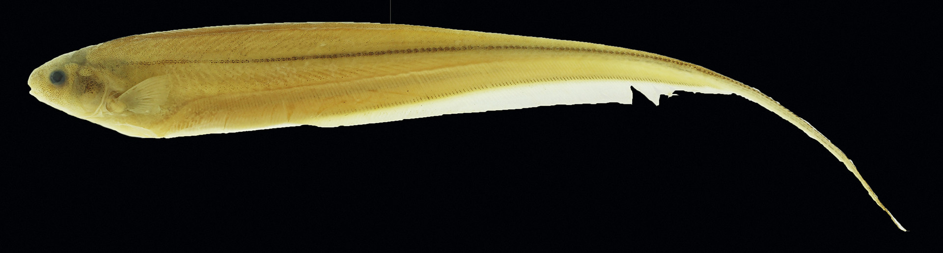
FIGURE 9| Holotype CZUT 11030 for Eigenmannia zenuensis, scale bar 1 cm.
Diagnosis. Eigenmannia zenuensis can be distinguished from congeners in the E. trilineata species group by the higher number of teeth in the dentary: 56-60 in 4-5 rows (vs. 8-15 in 1-2 rows in E. antonioi; 11-16 in 1-2 rows in E. muirapinima; 15-21 in 2 rows in E. pavulagem; 16 in 2 rows in E. microstomus; 16-18 in 2 rows in E. correntes; 17-18 in 2 rows in E. guairaca; 17-9 in 1-2 rows in E. loretana; 19-26 in 2 rows in E. sayona; 19-30 in 2-3 rows in E. besouro; 20-22 in 2 rows in E. camposi; 21-23 in 2 rows in E. desantanai; 23 in 2 rows in E. trilineata; 25-27 in 2 rows in E. matintapereira; 35-39 in 2-3 rows in E. magoi; 37-38 in 4 rows in E. waiwai and 38-45 in 3-4 rows in E. vicentespelaea).
Description. Morphometric and meristic data is shown in Tab. 9. Total Length (mm): 151.0-237.0. Ovoid scapular foramen. 69-86 vertebrae. 14-15 precaudal vertebrae. 31-34 premaxillary teeth in 4-5 rows. 7-11 endopterygoid teeth in 1-2 rows. 56-60 teeth in dentary in 4-5 rows. Scales small, cycloid, extending from immediately posterior of head to tip of caudal filament, presents. Suture between parietal and frontal bones serrated with similar teeth size. Posterior-most arm of the lateral ethmoid bone elongated and articulates with anterior-most prolongation of the frontal bone forming a window. Vomer with two extensions in base, forming groove with inverted crescent shape, posterolateral margins approximately the same width as parasphenoids. Width of anterior region of parasphenoid bone equal to width of both premaxillaries. Parasphenoid wide in anterior region; becomes narrower and forking posteriorly. Orbitosphenoid bone wide. Pterosphenoid bone wide. Posterior edge of the pterotic bone not completely rounded, has linear and non-curved edges. Posterior-most extension with right-angled triangular shape. Posterior base of basioccipital bone prolonged, bone itself not very round. Branchiostegal rays, 5 in total, 1-2 of same length, 3-5 with wide extensions, branchiosteal 4 the largest, sometimes branchiostegal 2 is large. Urohyal convex sheet reaches medial section of bone. Operculum upper edge rounded. Endopterygoid with long ascendant process. Basihyal length approximately 3/4 length of first ceratobranchial, slightly wider in anterior region, almost rectangular. Ceratobranchials with width conserved. 4-5 basibranchials, 2-3 well ossified. Four hypobranchials, first 3 well ossified. Upper pharyngeal tooth plate with 7 teeth. Lower pharyngeal tooth plate with 12 teeth. 9-10 cartilaginous gill rakers.
Coloration in alcohol. Background color pale cream to pale yellow. Head dark, darker than the rest of the body, darker in the dorsal region and lighter just by the dorsal region. Lips and suborbital region generally dark with concentrated chromatophores. Body with four visible dark stripes. Body darker above the lateral-line stripe. Lateral-line stripe dark, one scale deep, extending from the first perforated scale to the end of the caudal filament. Superior medial stripe wide, two scales deep, light brown color, extending from the posterior end of the gas bladder to a point approximately three-fourths of the body length from the snout. Inferior medial stripe with varying width, dark, blackish, originating near anus and extending to posterior end of the anal fin. Stripe along anal-fin base narrow, one to one and a half scales wide, dark brown color, extending along the edge of the anal fin. Pectoral fin hyaline with a few concentrated chromatophores around the base of the fin and in large individuals all along the fin. Anal fin hyaline, with some cases of few dispersed chromatophores along the base. Humeral spot present, not very dark, marking the beginning of the lateral-line stripe. Nape dark.
Geographic distribution. Eigenmanniazenuensis is known from the lower Magdalena, Cauca, and San Jorge rivers basins in Colombia (Fig. 7). This confluence area in the lowlands constitutes the most significant wetland in northern South America, known locally as the “Depresión Momoposina.”
Etymology. The specific epithet “zenuensis” is assigned in honor to the Amerindian Colombian tribe Zenú.
Discussion
Molecular and morphological data have questioned the monophyly of Eigenmannia (e.g., Alves-Gomes, 1998; Albert, 2001; Maldonado-Ocampo 2011). Dutra (2015), including in their analysis of eight valid Eigenmannia species and eight undescribed species (some of them currently described within the E. trilineata species group,) proposed two synapomorphies to support the monophyly of Eigenmannia: (1). The extension of the epipleural myorhabdoi bones over vertebrae 7-9; (2) The presence of an obliquus inferioris muscle limiting the posteroventral margin of the muscular hiatus between the first rib and the second rib.
However, as described by Galindo-Cuervo (2019), the two characters described above from Dutra (2015) are not exclusive to Eigenmannia, insomuch as these two characters also occur in Sternopygus (Fig. 10). Moreover, we noted that the degree to which the epipleural myorhabdoi bones extend over vertebrae 7-9 varies between species in both Eigenmannia and Sternopygus. For example, in E. camposi the epipleural myorhabdoi bones extend until vertebrae 6 and in E. humboldtii until vertebrae 9(Fig. 10). Also, the obliquus inferioris muscle limiting the posteroventral margin of muscular hiatus is between the fifth and sixth rib in E. camposi and between the fourth and fifth rib in E. humboldtii (Fig. 10). Based on these observations, Eigenmannia evidently still lacks unambiguous diagnostic characters common to all congeners. Consequently, the three new species described herein are provisionally assigned as members of Eigenmannia based on the absence of almost all diagnostic characters proposed for the remaining genera withinEigenmanniinae.
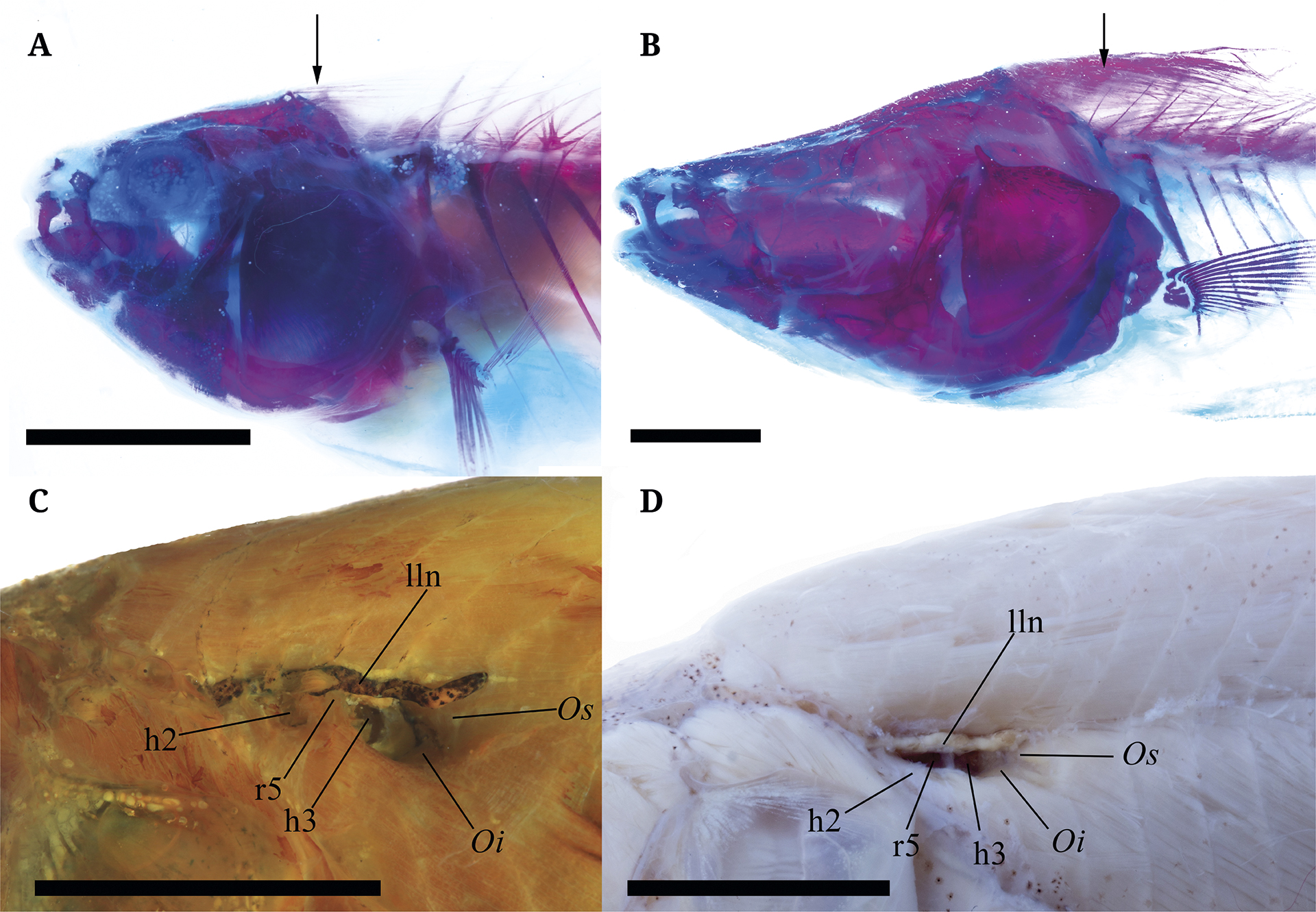
FIGURE 10| Morphology of myorhabdoi and pseudotympanum of Eigenmannia camposi (A.,C.; IAvH-P-7023) and Sternopygus aequilabiatus (B.,D.; MPUJ-9518) from the middle Magdalena basin (Honda-Tolima). A.E. camposi epipleural myorhabdoi bones. B.S. aequilabiatus epipleural myorhabdoi bones. C. Detail of the obliquus inferioris muscle limiting the posteroventral margin of muscular hiatus in E. camposi. D. Detail of the obliquus inferioris muscle limiting the posteroventral margin of muscular hiatus in S. aequilabiatus. Scale bar 1 cm.
The three new species described herein are included in the E. trilineata species group based on the presence of the superior medial stripe on the flank, a character considered to be a synapomorphy supporting this species group (Peixoto et al., 2015). Nonetheless, we acknowledge that the monophyly of the E. trilineata species group, as proposed by Peixoto et al. (2015), was not recovered in two phylogenetic studies that included some of the species of this species group: Dutra (2015) based on morphological characters, and Maldonado-Ocampo (2011) based on molecular characters.
Comparative examined material.Colombia: Eigenmannia humboldtii: ICN-MHN 16306, 4, 96.0-113.0 mm LEA. IAvH-P 7415, 5, 242.0-334.0 mm LEA. IAvH-P 9237, 1, 331.0 mm LEA. MPUJ 13408, 1, 257.0 mm LEA. MPUJ 13409, 1, 263.0 mm LEA. MPUJ 13410, 1, 282.0 mm LEA. MPUJ 13411, 1, 287.0 mm LEA. MPUJ 13412, 1, 263.0 mm LEA. Eigenmannia virescens: CZUT-IC X, 12, 86.0-255.0 mm LEA.
Key to species of the “Eigenmannia trilineata” species group
1a Number of premaxillary teeth 27-40 ……………….. 2
1b Number of premaxillary teeth 8-26 ……………….. 7
2a Number of premaxillary teeth 27 ……………….. 3
2b Number of premaxillary teeth 32-40 ……………….. 4
3a Suborbital depth 18 3-14 8% HL ……………….. Eigenmannia besouro
3b Suborbital depth 30-37 7% HL ……………….. Eigenmannia camposi n sp
4a Number of premaxillary teeth 32 ……………….. 5
4b Number of premaxillary teeth 35-40 ……………….. Eigenmannia wawai
5a Number of teeth in dentary 23 ……………….. Eigenmannia trilineata
5b Number of teeth in dentary 35-60 ……………….. 6
6a Number of teeth in dentary 35-39 ……………….. Eigenmannia magoi n sp
6b Number of teeth in dentary 56-60 ……………….. Eigenmannia zenuensis n sp
7a Number of premaxillary teeth 17-26 ……………….. 8
7b Number of premaxillary teeth 8-16 ……………….. 9
8a Number of teeth in dentary 16-18 ……………….. Eigenmannia correntes
8b Number of teeth in dentary 19-26 ……………….. 14
9a Number of endopterygoid teeth 5-7 ……………….. 10
9b Number of endopterygoid teeth 8-16 ……………….. 11
10a Orbital diameter 11 4-15 0 HL ……………….. Eigenmannia loretana
10b Orbital diameter 15 7-23 9 HL ……………….. Eigenmannia guairaca
11a Oral width 10 HL 19% HL ……………….. 12
11b Oral width 20 HL 25 1% HL ……………….. Eigenmannia antonioi
12a Suborbital depth 18-28 ……………….. 13
12b Suborbital depth 29 9-40 8 ……………….. Eigenmannia microstoma
13a Number of premaxillary teeth 8-10 ……………….. Eigenmannia muirapinima
13b Number of premaxillary teeth 13-16 ……………….. Eigenmannia pavulagem
14a First basibranchial ossified ……………….. Eigenmannia sayona
14b First basibranchial unossified ……………….. 15
15a Precaudal vertebrae 11-12 ……………….. Eigenmannia desantanai
15b Precaudal vertebrae 13-15 ……………….. 16
16a Precaudal vertebrae 13 ……………….. Eigenmannia matintapereira
16b Precaudal vertebrae 15 ……………….. Eigenmannia vicentespelaea
Acknowledgments
We dedicate this contribution to our esteemed mentor and co-author, Javier A. Maldonado-Ocampo, who died tragically during a field expedition in 2019. This work was supported by the Division of Research of the Pontificia Universidad Javeriana (Grant numbers: 00006305, 00006714 and 00007225) to J.A.M.O. The authors thank to Ricardo Campos-da-Paz and two anonymous reviewers for comments on the manuscript. The following provided support in field work and museum visits: Saúl Prada Pedreros and the Ichthyology Laboratory (MPUJ), José Iván Mojica and the Ichthyology group (ICN-MHN), Carlos DoNascimiento, Juan Albornóz and Alejandro Méndez (IAvH-P), Francisco Villa and Jaider Peña (CZUT), Ruth Gisela Reina, Rigoberto González and María Fernanda Castillo (STRI), Myreya Pinedo and Dimitri Forero (PUJ). JAMO would have wished to express his gratitude to James Albert, Nathan Lovejoy, William Crampton and José Alves Gomes for fruitful discussions about Gymnotiformes and to Rigoberto González for information about Panamanian Gymnotiformes.
References
Albert JS, Crampton WGR. Diversity and phylogeny of Neotropical electric fishes (Gymnotiformes). In: Bullock TH, Hopkins CD, Popper AN, Fay RR, editors. Electroreception. New York: Springer; 2006. p.360–409. https://doi.org/10.1007/0-387-28275-0_13
Albert JS, Reis RE. Historical biogeography of neotropical freshwater fishes. California: University of California Press; 2011.
Alves-Gomes JA. The phylogenetic position of the South American electric fish genera Sternopygus and Archolaemus (Ostariophysi, Gymnotiformes) according to 12S and 16S mitochondrial DNA sequences. In: Malabarba LR, Reis RE, Vari RP, Lucena ZMS, Lucena CAS, editors. Phylogeny and classification of Neotropical fishes. Porto Alegre: Edipucrs; 1998. p.447–60.
Baldwin CC, Mounts JH, Smith DG, Weigt LA. Genetic identification and color descriptions of early life-history stages of Belizean Phaeoptyx and Astrapogon (Teleostei: Apogonidae) with comments on identification of adult Phaeoptyx. Zootaxa. 2009; 2008:1–22.
Bookstein FL. Morphometric tools for landmark data: geometry and biology. New York: Cambridge University Press; 1991. http://dx.doi.org/10.11646/zootaxa.2008.1.1
Darriba D, Taboada GL, Doallo R, Posada D. jModelTest 2: more models, new heuristics and parallel computing. Nat Methods. 2012; 9(8):772. https://doi.org/10.1038/nmeth.2109
Dingerkus G, Uhler LD. Enzyme clearing of alcian blue stained whole small vertebrates for demonstration of cartilage. Biotech Histochem. 1977; 52(4):229–32. https://doi.org/10.3109/10520297709116780
Drummond AJ, Rambaut A. BEAST: Bayesian evolutionary analysis by sampling trees. BMC Evol Biol. 2007; 7(1):214. https://doi.org/10.1186/1471-2148-7-214
Dryden IL, Mardia KV. Statistical Shape Analysis: With Applications in R. Hoboken: John Wiley & Sons; 2016.
Dutra GM. Sistemática de Eigenmanniinae (Teleostei: Gymnotiformes: Sternopygidae). [PhD Thesis]. Belém: Museu Paraense Emílio Goeldi; 2015.
Dutra GM, de Santana CD, Wosiacki WB. A new species of the glass electric knifefish genus Eigenmannia Jordan and Evermann (Teleostei: Gymnotiformes: Sternopygidae) from Río Tuíra Basin, Panama. Copeia. 2017; 105(1):85–91. https://doi.org/10.1643/CI-16-439
Dutra GM, de Santana CD, Vari RP, Wosiacki WB. The South American electric glass knifefish genus Distocyclus (Gymnotiformes: Sternopygidae): Redefinition and revision. Copeia. 2014; (2):345–54. https://doi.org/10.1643/CI-13-066
Eslami A, Qannari EM, Bougeard S, Sanchez G. Package ‘multigroup’: Multigroup Data Analysis. Version 0.4.4. [Internet]. 2015. Available from: https://cran.r-project.org/web/packages/multigroup
Fujisawa T, Barraclough TG. Delimiting species using single-locus data and the Generalized Mixed Yule Coalescent approach: a revised method and evaluation on simulated data sets. Syst Biol. 2013; 62(5):707–24. https://doi.org/10.1093/sysbio/syt033
Galindo-Cuervo A. Anatomía comparada de huesos, músculos, órgano eléctrico y su descarga en especies trans andinas de la familia Sternopygidae. [PhD Thesis]. Bogotá: Pontificia Universidad Javeriana; 2019.
Hall T. BioEdit: An important software for molecular biology. GERF Bull Biosc. 2011; 2(1):60–61.
Hopkins CD. Electric communication in the reproductive behavior of Sternopygus macrurus (Gymnotoidei). Z Tierpsychol. 1974; 35:518–35. https://doi.org/10.1111/j.1439-0310.1974.tb00465.x
Hulen K.G., Crampton W.G.R & Albert, J.S. Phylogenetic systematics and historical biogeography of the Neotropical electric fish Sternopygus (Teleostei: Gymnotiformes), Systematics and Biodiversity. 2005; 3:4, 407-32. https://doi.org/10.1017/S1477200005001726
Kumar S, Stecher G, Tamura K. MEGA7: Molecular Evolutionary Genetics Analysis version 7.0 for bigger datasets. Mol Biol Evol. 2016; 33(7):1870–74. https://doi.org/10.1093/molbev/msw054
Mago-Leccia F. Los peces de la familia Sternopygidae de Venezuela. Incluyendo una description de la osteologia de Eigenmannia virescens y una nueva definicion y classificacion del orden Gymnotiformes. Acta Cient Venez. 1978; 29(1):1–89.
Maldonado-Ocampo JA. Filogenia molecular da família Sternopygidae (Gymnotiformes: Sternopygoidei). [PhD Thesis]. Rio de Janeiro: Universidade Federal do Rio de Janeiro; 2011.
Maldonado-Ocampo JA, Albert JS. Species diversity of gymnotiform fishes (Gymnotiformes, Teleostei) in Colombia. Biota Colomb. 2003; 4(2):147–65. Available from: http://www.redalyc.org/articulo.oa?id=49140202
Matamoros WA, McMahan CD, Chakrabarty P, Albert JS, Schaefer JF. Derivation of the freshwater fish fauna of Central America revisited: Myers’s hypothesis in the twenty-first century. Cladistics. 2015; 31(2):177–88. https://doi.org/10.1111/cla.12081
Peixoto LAW, Dutra GM, Wosiacki WB. The electric glass knifefishes of the Eigenmannia trilineata species-group (Gymnotiformes: Sternopygidae): monophyly and description of seven new species. Zool J Linn Soc. 2015; 175(2):384–414. https://doi.org/10.1111/zoj.12274
Peixoto LAW, Ohara WM. A new species of Eigenmannia Jordan & Evermann (Gymnotiformes: Sternopygidae) from rio Tapajós, Brazil, with discussion on its species group and the myology within Eigenmanniinae. PLoS One. 2019; 14(8):e0220287. https://doi.org/10.1371/journal.pone.0220287
Pons J, Barraclough TG, Gomez-Zurita J, Cardoso A, Duran DP, Hazell S, Kamoun S, Dumlin WD, Vogler AP. Sequence-based species delimitation for the DNA taxonomy of undescribed insects. Syst Biol. 2006; 55(4):595–609. https://doi.org/10.1080/10635150600852011
Puillandre N, Lambert A, Brouillet S, Achaz G. ABGD, Automatic Barcode Gap Discovery for primary species delimitation. Mol Ecol. 2012; 21(8):1864–77. https://doi.org/10.1111/j.1365-294X.2011.05239.x
Raikow RJ, Bledsoe AH, Myers BA, Welsh CJ. Individual Variation in Avian Muscles and its Significance for the Reconstruction of Phylogeny. Syst Biol. 1990; 39(4):362–70. https://doi.org/10.2307/2992356
Rambaut A, Drummond AJ. TreeAnnotator. Version 1.8.2 [Internet]. Edinburgh: University of Edinburgh; 2016. Available from: http://beast.community/treeannotator
Rambaut A, Suchard MA, Xie D, Drummond AJ. Tracer. Version 1.6 [Internet]. Edinburgh: University of Edinburgh; 2014. Available from http://beast.community/tracer
Rohlf FJ. TpsDig2. Version 2.26. [Internet]. Stony Brook: The State University of New York; 2016a. Available from: http://life.bio.sunysb.edu/morph
Rohlf FJ. TpsUtil. Version 1.70. [Internet]. Stony Brook: The State University of New York; 2016b. Available at http://life.bio.sunysb.edu/morph
De Santana CD, Crampton WGR, Dillman CB, Frederico RG, Sabaj MH, Covain R, Ready JS, Zuanon J, Oliveira RR, Mendes-Júnior RNG, Bastos DA, Teixeira TF, Mol J, Ohara WM, Castro NC, Peixoto LA, Nagamachi C, Sousa LM, Montag LFA, Ribeiro FR, Waddell JC, Piorsky NM, Vari RP, Wosiacki WB. Unexpected species diversity in electric eels with a description of the strongest living bioelectricity generator. Nat Commun. 2019; 10(4000):1–10. https://doi.org/10.1038/s41467-019-11690-z
Schlick-Steiner BC, Steiner FM, Seifert B, Stauffer C, Christian E, Crozier RH. Integrative taxonomy: a multisource approach to exploring biodiversity. Annu Rev Entomol. 2010; 55:421–38. https://doi.org/10.1146/annurev-ento-112408-085432
Sheets HD. Software IMP (Integrated morphometrics package). Version 8.0. [Internet] Buffalo: Canisius College; 2004.
Tagliacollo VA, Bernt MJ, Craig JM, Oliveira C, Albert JS. Model-based total evidence phylogeny of Neotropical electric knifefishes (Teleostei, Gymnotiformes). Mol Phylogenet Evol. 2016; 95:20–33. https://doi.org/10.1016/j.ympev.2015.11.007
Xia X, Xie Z. DAMBE: software package for data analysis in molecular biology and evolution. J Hered. 2001; 92(4):371–73. https://doi.org/10.1093/jhered/92.4.371
Zelditch ML, Swiderski DL, Sheets HD. Geometric morphometrics for biologists: a primer. London: Academic Press; 2012.
Zhang J, Kapli P, Pavlidis P, Stamatakis A. A general species delimitation method with applications to phylogenetic placements. Bioinformatics. 2013; 29(22): 2869–76. https://doi.org/10.1093/bioinformatics/btt499
Authors

![]() Edgar Esteban Herrera-Collazos1,
Edgar Esteban Herrera-Collazos1, ![]() Aleidy M. Galindo-Cuervo1,
Aleidy M. Galindo-Cuervo1, ![]() Javier A. Maldonado-Ocampo1† and
Javier A. Maldonado-Ocampo1† and ![]() Melissa Rincón-Sandova1
Melissa Rincón-Sandova1 ![]()
[1] Laboratorio de Ictiología, Unidad de Ecología y Sistemática (UNESIS), Departamento de Biología, Facultad de Ciencias, PontificiaUniversidad Javeriana, Carrera 7, N° 43-82, 110231561 Bogotá, D.C., Colombia. (EEHC) edgarestebanhc@gmail.com; (AMG) aleidy.galindo@javeriana.edu.co; (JAMO) maldonadoj@javeriana.edu.co ( deceased); (MRS) melissarincons@gmail.com
Authors’ Contribution 

Edgar E. Herrera-Collazos: Conceptualization, Data curation, Formal Analysis, Investigation, Methodology, Resources, Software, Validation, Visualization, Writing (original draft).
Aleidy M. Galindo-Cuervo: Investigation, Methodology, Formal analysis, Validation, Writing (original draft), Writing (review & editing).
Javier A. Maldonado-Ocampo: Conceptualization, Funding acquisition, Investigation, Project administration, Resources, Supervision, Writing (original draft).
Melissa Rincón-Sandoval: Data curation, Formal Analysis, Investigation, Methodology, Software, Validation, Visualization, Writing (original draft), Writing (review & editing).
Competing Interests
Not applicable.
How to cite this article
Herrera-Collazos EE, Galindo-Cuervo AM, Maldonado-Ocampo JA, Rincón-Sandoval M. Three new species of the Eigenmannia trilineata species group (Gymnotiformes: Sternopygidae) from northwestern South America. Neotrop Ichthyol. 2020; 18(1):e180085. https://doi.org/10.1590/10.1590/1982-0224-2018-0085
Copyright
This is an open access article under the terms of the Creative Commons Attribution License, which permits use, distribution and reproduction in any medium, provided the original work is properly cited.
Distributed under
Creative Commons CC-BY 4.0

© 2020 The Authors.
Diversity and Distributions Published by SBI
![]() Accepted February 17, 2020 by William Crampton
Accepted February 17, 2020 by William Crampton
![]() Submitted June 21, 2018
Submitted June 21, 2018
![]() Epub April 20, 2020
Epub April 20, 2020